Recently the MNIST image set was examined with some popular machine learning algorithms (including logistic regression, random forests, and xgBoost). This time a simple neural network is used to perform the classification.
There is quite a bit of information about neural networks out there already, so the background information is being largely omitted. The key thing is that a neural network structures and processes data in a manner similar to the way a human brain operates.
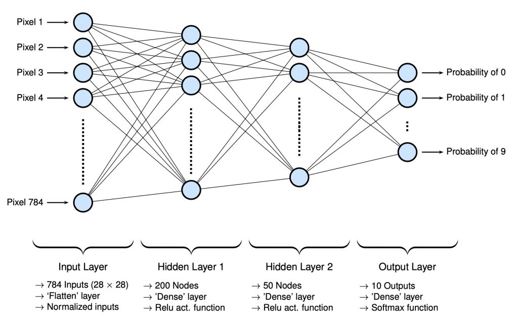
For the MNIST dataset, a simple neural network can be used to classify the handwritten numbers with better accuracy than the previously used ML algorithms. A simple network with two hidden layers was used where chosen number of nodes for each layer was based on some reasonable values from past experiences (note that they can be altered a bit to achieve similar results). The input layer takes a normalized version of the image values in a flattened format. The output layer reports results using the softmax function. Below is a rough schematic of the architecture of the network. Note that it is abbreviated in that not all nodes are shown; since over 1000 would have to be drawn, only a few are drawn to convey the general message.
Building a Network with TensorFlow2 and Keras
To build the above network it is very easy using Keras with TensorFlow2 with the following code:
import tensorflow as tf
from tensorflow import keras

model = keras.Sequential ()
model.add (keras.layers.Flatten (input_shape=[28,28]))
model.add (keras.layers.Dense (units = 200, activation = 'relu'))
model.add (keras.layers.Dense (units = 50, activation = 'relu'))
model.add (keras.layers.Dense (units = 10, activation = 'softmax'))

model.compile (optimizer = 'Nadam', loss = 'sparse_categorical_crossentropy', metrics=['accuracy'])
A few things to note… in the input layer the size is based on the number of pixel of each input image (which are 28 x 28). The sparse_categorical_crossentropy loss function is needed since the output layer is using softmax as its activation function.
The summary function can be used to view a summary of the model’s architecture to make sure things were properly created:
model.summary ()

Model: "sequential"
_________________________________________________________________
Layer (type)                 Output Shape              Param #
=================================================================
flatten (Flatten)            (None, 784)               0
_________________________________________________________________
dense (Dense)                (None, 200)               157000
_________________________________________________________________
dense_1 (Dense)              (None, 50)                10050
_________________________________________________________________
dense_2 (Dense)              (None, 10)                510
=================================================================
Total params: 167,560
Trainable params: 167,560
Non-trainable params: 0
_________________________________________________________________
Recall that each node contains n weight values for each input from the previous layer, along with one bias value. Therefore the number of parameters is explained as:
It is pretty remarkable, that various neural network algorithms can work out all of these weight and bias parameters pretty quickly with a high degree of accuracy.
Training and Evaluating the Network
First we need to get the data, which is an easy process since it is distributed with tensorflow. After that it will be split into training, validation, and test sets. Note that the training data needs to be normalized so that the model can converge quicker.
# load the data...
(x_train_all, y_train_all), (x_test, y_test) = keras.datasets.mnist.load_data ()

x_valid = x_train_all [:VALIDATION_SET_SIZE] / 255.0
x_train = x_train_all [VALIDATION_SET_SIZE:] / 255.0

y_valid = y_train_all [:VALIDATION_SET_SIZE]
y_train = y_train_all [VALIDATION_SET_SIZE:]

x_test  = x_test / 255.0
Training is very simple. The fit function can be just called on the training data. Note that at the end of each epoch, the current state of the model can be evaluated using the supplied validation data. For the MNIST dataset, for an acceptable level of accuracy at least 15 epochs should be used.
trainHistory = model.fit (x_train, y_train, epochs = EPOCHS, validation_data = (x_valid, y_valid))After 25 epochs, training results in a model with 99.77% accuracy (the accuracy using the validation set was 98.08%). Note that the fit function returns the accuracy and the outcome of the loss function for both the training and validation sets. Below is a graph of the accuracy change over the training process.
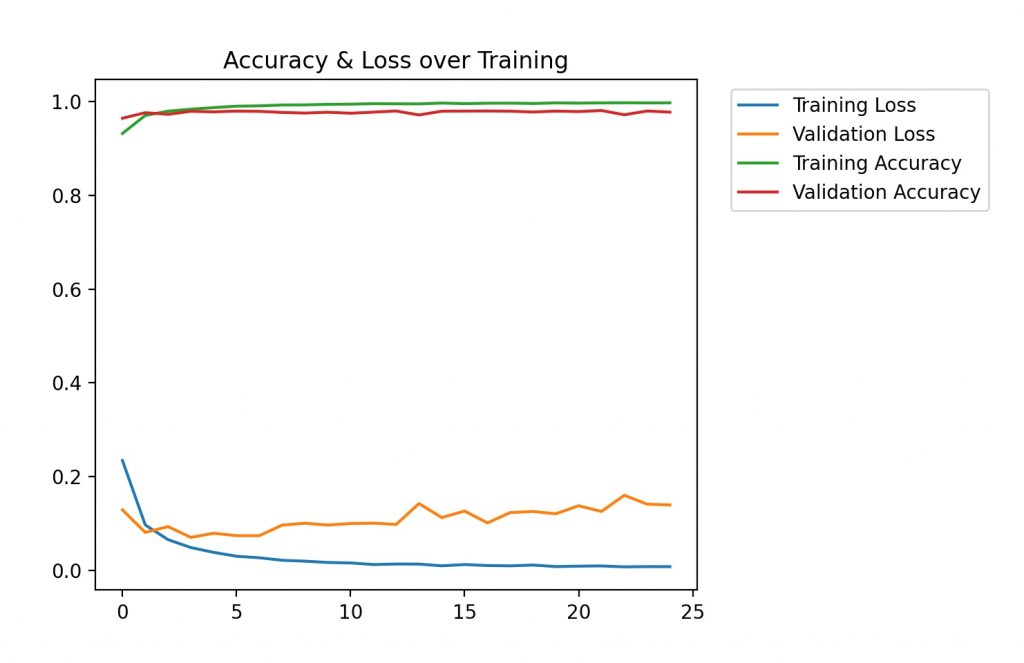
To evaluate the accuracy with the model with the test set, the evaluate function is called. In our case, model was 97.89% accurate with the test data.
results = model.evaluate (x_test, y_test)

313/313 [==============================] - 0s 1ms/step - loss: 0.1427 - accuracy: 0.9789
test loss, test acc:  [0.14265398681163788, 0.9789000153541565]
Building a Model for Testing…
Once a model is trained, in the same script (or notebook) it can be used to make some predictions. This is not the most efficient way of doing things since just to make some quick predictions one would have to suffer through the training process. A better way is train the model once and save it the results (all the weights and structure) to a file, and when a prediction needs to be made, load the model file first. It’s really easy to save the structure and weights of a model:
model.save (MODEL_OUTPUT_FILE)In a different script, to load (or build) the model its just as easy…
model = keras.models.load_model (MODEL_FILE)Predicting with my own Data…
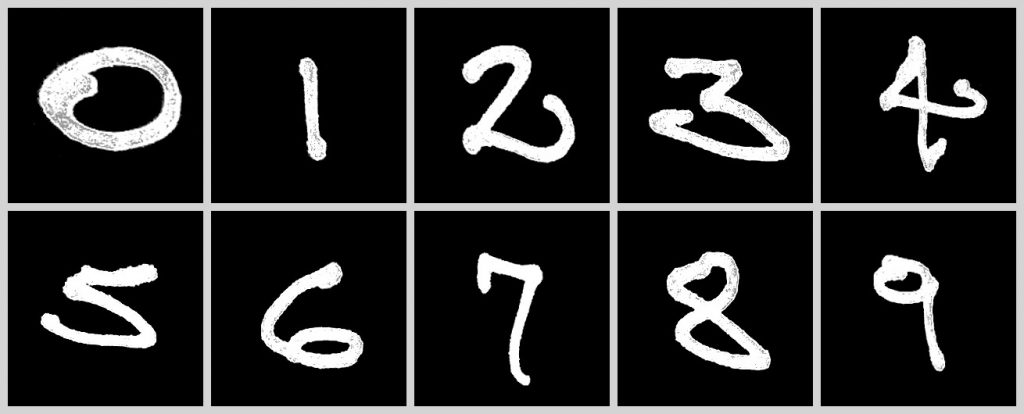
Instead of using any of the given values (from either from the testing, training, or validation sets), to keep things interesting the model was used to make predictions with my own handwritten numbers.
The numbers shown below all work successfully. However there was some problems along the way; some items to note when using one’s own handwritting:
- The numbers need to take the majority of the space of the image (or around three-quarters of it). If they are too small/larger a lot of incorrect predictions will occur
- Also, the numbers need to be in a style similar to the others in the set. That is, nothing to artistic or wacky can be used
- Finally, the numbers shouldn’t be too bright or too dark. This is less of an issue, but it should still be noted.
Steps Required…
To use one’s own handwriting:
- First make sure a number takes three quarters of a square image and isn’t too dark/light in brightness/contrast.
- Resize the image to be 28 x 28 in size and save it to an 8-bit gray scale PNG file.
Next, in the code the image needs to be prepared for the model. That is the model was trained with images in a particular style so the image need to be modified so it is in the same style. Basically, it will be normalized and extra empty dimensions will added.
def prepImage (img, imgSize):

    # first convert it to a np array from a PIL image
    img = np.array (img)

    # from 28 x 28 to 28 x 28 x 1
    img = tf.expand_dims (img, -1)

    # next normalize it
    img = tf.divide (img, 255)

    # resize to the input of the pretrained neural net.
    img = tf.image.resize (img, [imgSize, imgSize])

    # reshape to add batch dimension
    img = tf.reshape(img, [1, imgSize, imgSize, 1])

    return img
To make a prediction, the predict function is simply called…
preds = model.predict (img)The predict function returns a list of probabilities for each labelled possible number. As a nice coincidence, there is a direct correspondence with the order of the probabilities and the value of the number. Hence the predicted value is simply the index of the max probability:
label = np.argmax (preds)Results…
Again, the results were all successful. The majority of the numbers had 100% predictions. That is, 0, 5, 7, and 8, all had similar results to 9:
0 --> 3.037e-21 %
1 --> 1.118e-10 %
2 --> 2.513e-14 %
3 --> 3.884e-06 %
4 --> 5.459e-09 %
5 --> 4.303e-08 %
6 --> 1.313e-25 %
7 --> 2.174e-09 %
8 --> 5.567e-10 %
9 --> 100.0 %
For the remaining values, the predictions were still in the upper 90s. For example with 4 we had:
0 --> 1.46e-15 %
1 --> 0.6095 %
2 --> 2.995e-13 %
3 --> 1.469e-09 %
4 --> 99.33 %
5 --> 6.89e-09 %
6 --> 0.05974 %
7 --> 1.32e-05 %
8 --> 4.42e-05 %
9 --> 1.992e-11 %
Code…
All the code used along with the test images is available here.
No Comments