Previously the MNIST dataset was used in the examination of different classification techniques. This includes a variety of machine learning algorithms (including random forests, logistic regression, and xgboost), and simple neural networks. This time around, a few convolutional neural networks will be used to conclude the experiments with MNIST classifiers.
Convolutional neural networks (or CNNs) contain a few additional layers compared to other simple neural networks; namely 2D convolutional filter and (max) pooling layers. The 2D convolutional filter layers applies multiple convolution kernels to an input image to emphasize local patterns. The pooling layers reduce the size of the image by focusing on the most important pixels and discarding the rest.
Since the MNIST dataset is pretty simple, three pretty straightforward CNNs were made to gain some experience using them to classify images.
CNN 1: Fundamental CNN
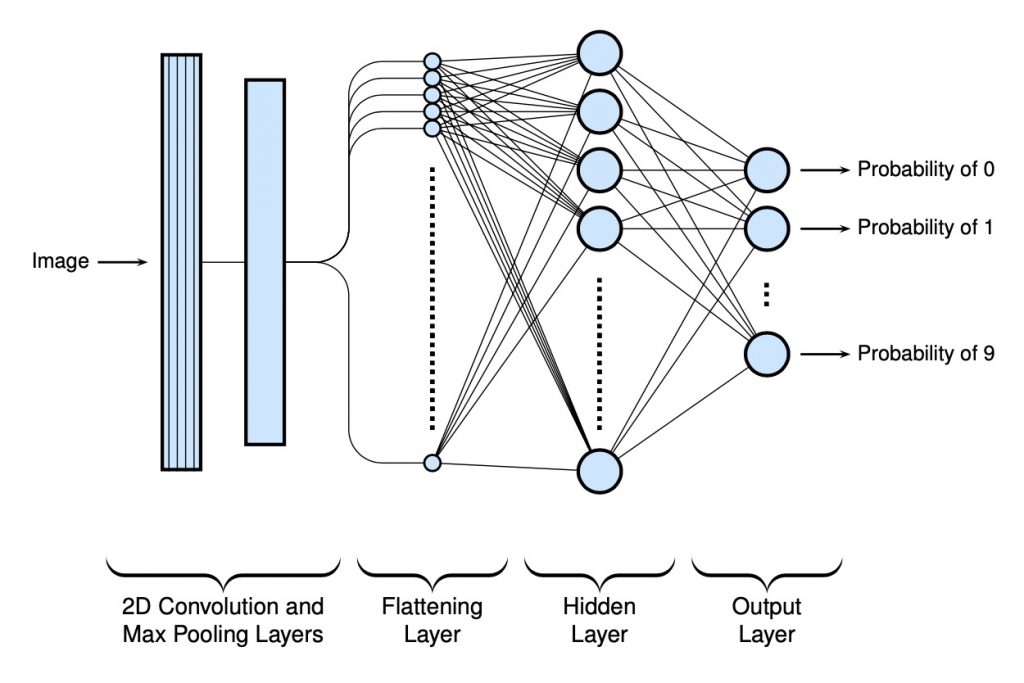
For the first CNN, a 2D convolutional layer and max pooling layer have been added at the beginning of the model to help find some local patterns with the pixels. For the filters, 32 3 \times convolutional kernel matrices are used (with no additional padding). The max pooling will scale the image down by a factor of 2. Below is a high level schematic of the model (in a manner that only makes sense for myself):
Below is the code used to build the model…
model.add (layers.Conv2D(32, (3, 3), activation='relu', kernel_initializer='he_uniform', input_shape=INPUT_SHAPE))
model.add (layers.MaxPooling2D((2, 2)))
model.add (layers.Flatten())
model.add (layers.Dense(100, activation='relu', kernel_initializer='he_uniform'))
model.add (layers.Dense(10, activation='softmax'))

opt = keras.optimizers.SGD (lr=0.01, momentum=0.9)
model.compile(optimizer=opt, loss='categorical_crossentropy', metrics=['accuracy'])
And the output from model.summary():
Model: "sequential"
_________________________________________________________________
Layer (type)                 Output Shape              Param #
=================================================================
conv2d (Conv2D)              (None, 26, 26, 32)        320
_________________________________________________________________
max_pooling2d (MaxPooling2D) (None, 13, 13, 32)        0
_________________________________________________________________
flatten (Flatten)            (None, 5408)              0
_________________________________________________________________
dense (Dense)                (None, 100)               540900
_________________________________________________________________
dense_1 (Dense)              (None, 10)                1010
=================================================================
Total params: 542,230
Trainable params: 542,230
Non-trainable params: 0
_________________________________________________________________
This model took around 4 minutes to train, and had an accuracy of 98.7% with the test set.
CNN 2: Fundamental with Batch Normalization
The first CNN did have some good results, however a small change was added to it to further improve the results. While the MNIST dataset is more of a toy dataset and the network is fairly shallow, it is still good to experiment a bit with the model.
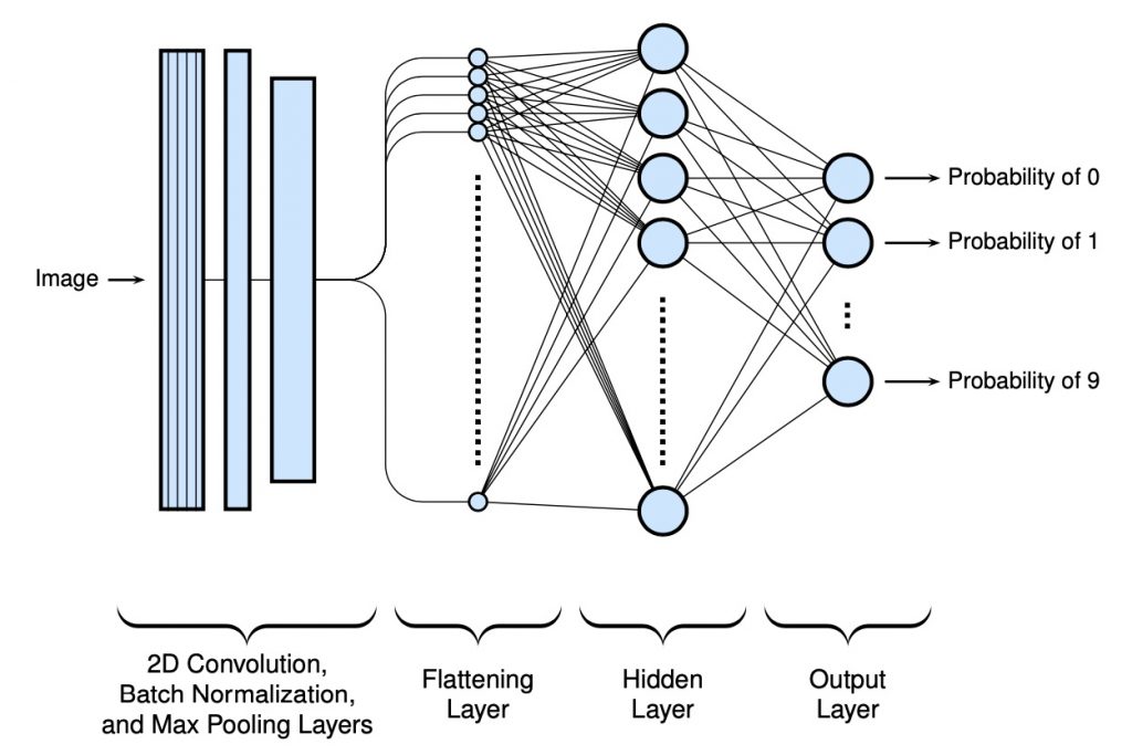
In this case, a batch normalization layer was added to speed up convergence (and escape any plateaus) during training. A high level view of the model is shown below:
and the code to create this model…
model.add (layers.Conv2D(32, (3, 3), activation='relu', kernel_initializer='he_uniform', input_shape=INPUT_SHAPE))
model.add (layers.BatchNormalization())
model.add (layers.MaxPooling2D((2, 2)))
model.add (layers.Flatten())
model.add (layers.Dense(100, activation='relu', kernel_initializer='he_uniform'))
model.add (layers.Dense(10, activation='softmax'))

opt = keras.optimizers.SGD (lr=0.01, momentum=0.9)
model.compile(optimizer=opt, loss='categorical_crossentropy', metrics=['accuracy'])
and the output from model.summary():
Model: "sequential"
_________________________________________________________________
Layer (type)                 Output Shape              Param #
=================================================================
conv2d (Conv2D)              (None, 26, 26, 32)        320
_________________________________________________________________
batch_normalization (BatchNo (None, 26, 26, 32)        128
_________________________________________________________________
max_pooling2d (MaxPooling2D) (None, 13, 13, 32)        0
_________________________________________________________________
flatten (Flatten)            (None, 5408)              0
_________________________________________________________________
dense (Dense)                (None, 100)               540900
_________________________________________________________________
dense_1 (Dense)              (None, 10)                1010
=================================================================
Total params: 542,358
Trainable params: 542,294
Non-trainable params: 64
_________________________________________________________________
This model took slightly more than 4 minutes to train to get to the same level accuracy 98.6% as before (with the test set). The big difference is that each training set took longer but less overall steps were needed since the model converged quicker. Note that early stopping was used during training with a delta value of 0.01.
CNN 3: Multiple Conv2D Layers
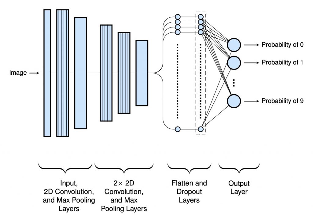
Finally, a slightly more deep model was used with extra convolutional layers (1 with 32 and 2 with 64 filters each). These find a higher degree of patterns with the pixels. To reduce the chance of overfitting, a dropout layer was included (with a dropout value of 0.5). Note that no standard or classical hidden dense layers have been added. Below is an example schematic of the final network (again in my homemade style):
The code used to make the model…
model.add (keras.Input (shape=INPUT_SHAPE))
model.add (layers.Conv2D (32, kernel_size=(3, 3), activation='relu'))
model.add (layers.MaxPooling2D (pool_size=(2, 2)))
model.add (layers.Conv2D (64, kernel_size=(3, 3), activation='relu'))
model.add (layers.Conv2D (64, kernel_size=(3, 3), activation='relu'))
model.add (layers.MaxPooling2D (pool_size=(2, 2)))
model.add (layers.Flatten ())
model.add (layers.Dropout (0.5))
model.add (layers.Dense (NUM_CLASSES, activation='softmax'))

model.compile (loss='categorical_crossentropy', optimizer='adam', metrics=['accuracy'])
and the output from model.summary():
Model: "sequential"
_________________________________________________________________
Layer (type)                 Output Shape              Param #
=================================================================
conv2d (Conv2D)              (None, 26, 26, 32)        320
_________________________________________________________________
max_pooling2d (MaxPooling2D) (None, 13, 13, 32)        0
_________________________________________________________________
conv2d_1 (Conv2D)            (None, 11, 11, 64)        18496
_________________________________________________________________
conv2d_2 (Conv2D)            (None, 9, 9, 64)          36928
_________________________________________________________________
max_pooling2d_1 (MaxPooling2 (None, 4, 4, 64)          0
_________________________________________________________________
flatten (Flatten)            (None, 1024)              0
_________________________________________________________________
dropout (Dropout)            (None, 1024)              0
_________________________________________________________________
dense (Dense)                (None, 10)                10250
=================================================================
Total params: 65,994
Trainable params: 65,994
Non-trainable params: 0
_________________________________________________________________
This model took slightly more than double the amount of time of the previous two models (around 9.5 minutes). However, the accuracy was better (99.4%) and the number of variables used was significantly reduced with just 12% of what was used with the first models.
Summary of Results…
| Network | Number of Trainable Parameters |
Accuracy | Average Time per Epoch |
Total Time Used |
Epochs Required |
| 1 | 542,230 | 98.7 | 20.7 | 231.191 | 11 |
| 2 | 542,294 | 98.6 | 26.3 | 264.893 | 9 |
| 3 | 65,994 | 99.40 | 46.1 | 565.271 | 12 |
Code…
All of the code is available here.
No Comments