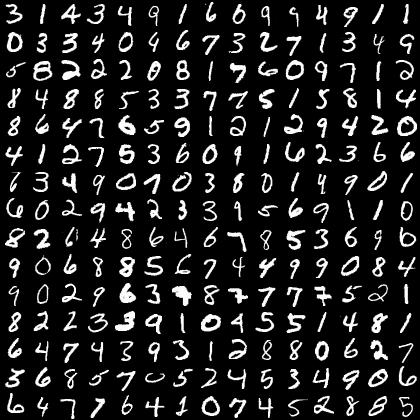
This project is more of a ‘Hello World’ type of project in the world of machine learning and image processing. The MNIST dataset is a set of 70,000 images (that is 60,000 for training and 10,000 for testing) of handwritten digits of from 0 to 9. The MNIST images is perhaps one of the better supervised learning datasets, that is all images have been labelled with the corresponding numeric value that it represents. It is a good dataset to compare various classification algorithms and gain some exposure to machine learning. Below is an image of a sample of the first few images from the dataset…
For this project some of the more traditional algorithms were used to ‘classify’ the dataset. Classification is the process of training a mathematical model on part of the dataset (the training set), and then using the model to make predictions of the class type on unseen data.
This little project of some of the more basic algorithms is to act as more of a ‘stepping stone’ in the domain of machine learning and imaging processing. The next steps include using a standard neural network (with the softmax function) and then using a convolutional neural network, both with the same dataset.
Simplest Case: Single Number Classification…
The simplest case is a binary classification problem; that is the goal is to make a model that can predict if something is a member of a set or not. Therefore, we shall train a model to ‘learn’ if a number is a member of a particular set or not (for example the set of 5 versus the set of everything other than a 5).
To keep things easy to manage, 4 of the simpler models were used. These models might not produce the greatest amount of precision, but they are easy to compute on an older machine. (Again, the purpose of this project is to act more of a stepping stone for future more complicated projects that use better techniques). The 4 models that were used include:
- Stochastic Gradient Descent : this is a simple linear classifier, but instead of computing a hyperplane of best fit with all the points, fitting is done with a randomly selected subset a small set of times.
- Random Forest : a set of decision trees are averaged together when making a prediction.
- Logistic Regression : logistic regression is perhaps the simplest go to when dealing with binary classification (at least for me).
- K-Neighbours : this is perhaps the best classifier of the ones chosen, but it is the most expensive to compute
But First… Loading the data…
Sci Kit Learn provides a nice tool to get and load the data. The fetch_openml function gets a copy of the dataset and then stores it locally; any future calls to the function uses the cached data. Below is the code needed to load and open the dataset.
from sklearn.datasets import fetch_openml
mnist = fetch_openml ('mnist_784', version=1)
Note that each image is a 28 x 28 8-bit greyscale image, so that 70,000 image results in approximately 55 Mbs. On a slower machine, the fetch call usually takes approximately 25 seconds to execute.
Creating the Test and Train Sets…
Next the data needs to be broken into two sets, one to train a model, and one to test out the trained model. The most common way is to split the dataset using a list’s split operator (:) with a fixed percentage (usually 10-20%, or preset value (say 10,000 values). SciKit-Learn comes with two functions which make this a bit easier: test_train_split does a simple split as mentioned and StratifiedShuffleSplit provides some randomness to the split along with keeping the same ratio of the various elements in the two produced sets. Note that the MNIST data is already in a random order so it does not need to be shuffled.
# First establish X and y...
X = mnist ['data']
y = mnist ['target']
y = y.astype (np.uint8)

# Then create test and train sets...
TRAIN_TEST_SPLIT = 10000
X_train, X_test = X[:(X.shape[0] - TRAIN_TEST_SPLIT)], X[(X.shape[0] - TRAIN_TEST_SPLIT):]
y_train, y_test = y[:(X.shape[0] - TRAIN_TEST_SPLIT)], y[(X.shape[0] - TRAIN_TEST_SPLIT):]
Since we are performing a binary classification, the labels (this is the y values) need to be adjusted from their original meaning to simply in the set (1 or True) and not in the set (0 or False). In our code, NUMBER is the specific number that we wish to classify.
y_train_N = (y_train == NUMBER)
y_test_N  = (y_test  == NUMBER)
Building and Training the Model…
Making and training the model is rather easy. All one needs to do is create an instance and call the fit function with the training data set.
Therefore to build the appropriate model…
from sklearn.linear_model import SGDClassifier
clf = SGDClassifier (random_state=42)

from sklearn.ensemble import RandomForestClassifier
clf = RandomForestClassifier (random_state=42, n_estimators=50)

from sklearn.linear_model import LogisticRegression
clf = LogisticRegression (solver='lbfgs', max_iter=1000, random_state=42)

from sklearn.neighbors import KNeighborsClassifier
clf = KNeighborsClassifier (weights='distance', n_neighbors=4)
Training the model…
clf.fit (X_train, y_train_N)Using the Model to Make Predictions…
With the trained model, the predict function can be called with elements from the test set to make predictions.
pred = clf.predict (X_test[i].reshape(1, -1))Using the results for each prediction, the model’s accuracy can be determined from some key measurements, namely:
- True Positives: the model predicts that a number is actually of the desired set of numbers.
- True Negatives: the model predicts that a number is not a member set of numbers.
- False Positives: numbers that the model incorrectly identified as a member of the desired set of numbers.
- False Negatives: numbers that the model should have identified as members of the desired set but did not.
The above measurements can be determined by simply counting and comparing results.
TruePos  = []
TrueNeg  = []
FalsePos = []
FalseNeg = []

for i in range (len(X_test)):
    predTest = clf.predict (X_test[i].reshape(1, -1))

    if predTest == True and y_test_N [i] == True:
        TruePos.append (i)
    elif predTest == False and y_test_N [i] == False:
        TrueNeg.append (i)
    elif predTest == True and y_test_N [i] == False:
        FalsePos.append (i)
    elif predTest == False and y_test_N [i] == True:
        FalseNeg.append (i)
Instead of looking at raw counts of predictions, new values can be determined that are percentages so that different models and results from different dataset can be compared. These are the precision and recall.
The precision is the ratio of the number of correct predictions versus the total amount of elements/numbers that were selected. It is calculated by:
The recall is the ratio of the correct predictions versus the total amount of possible elements/numbers in the set. It is calculated by:
The precision and recall can be combined together into one number which is referred to as the F1-Score. This allows a quick comparison between various models and datasets:
With the 4 different models and all the numbers (0 to 9), the complete results are summarized in the graph below (or click here to view it in a separate tab):
Just looking at the Stochastic Gradient Descent results we can a see some sample images of the true-positives, true-negatives, false-positives, and false-negatives below. Note for a few cases there are less than 36 elements which makes the resulting image look incomplete.
Validating the Model…
The precision and recall can be used to create a special plot called the ROC curve. Classification is based on a fixed cutoff threshold c (usually its 50%). However, the precision and recall can be determined for a variety of c values and then used in a plot. Note that instead of using the precision, the specificity is used which is calculated by:
Also note that depending on the user/textbook, many different names are often used, but they all mean the same thing, including:
- Recall: sensitivity or hit rate or true positive rate
- Specificity: selectivity or true negative rate
The main things with the ROC curve is:
- The closer the curve approaches the top left corner the better
- The closer the area under the curve (AUC) is to 1 the better
- It is a good way to compare different classifiers.
Overall Results…
Stochastic gradient descent is perhaps the easier to compute, however it isn’t the best classifier. K-neighbours is the best classifier by far with an accuracy rate of greater than 99%, however it is the more time consuming technique to compute.
Case 2: Classifying all Numbers…
To make a full classifier, that is one that compares each number with all others, a binary classifier can still be used, however it things get slightly complicated. Two possible strategies in doing so are:
- The one-versus-the-rest strategy (OvR) (or sometimes call one-versus-all). Here N different classifiers are created, with 1 for each number in the set (for MNIST 10 need to be created). During classification, a comparison is done between each classifier and the best score decides which group the value it belongs to.
- And the one-versus-one strategy (OvO); here a binary classifier is trained for every pair of image combination (for example, 0 and 1, 1 and 2, and so on…). For N classes, then \frac{1}{2} N(N – 1) combinations need to be trained. This is a better solution for smaller datasets.
Some algorithms scale poorly and hence the OvO strategy is preferred in those cases. SciKit Learn is nice since it have built in heuristics to choose the better strategy for the chosen algorithm. Simply calling the fit on a multi-labelled dataset will automatically perform multi-class classification with the correct strategy.
For our tests, the stochastic gradient descent classifier was used with the OvR strategy. It is not the best classifier, however it was chosen since more errors are present which can be further explored (again this is for learning purposes). Also it is perhaps one of the quickest techniques to calculate. In the code, things are pretty simple…
X_train, X_test = X[:(X.shape[0] - TRAIN_TEST_SPLIT)], X[(X.shape[0] - TRAIN_TEST_SPLIT):]
y_train, y_test = y[:(X.shape[0] - TRAIN_TEST_SPLIT)], y[(X.shape[0] - TRAIN_TEST_SPLIT):]
clf = SGDClassifier (random_state=42)
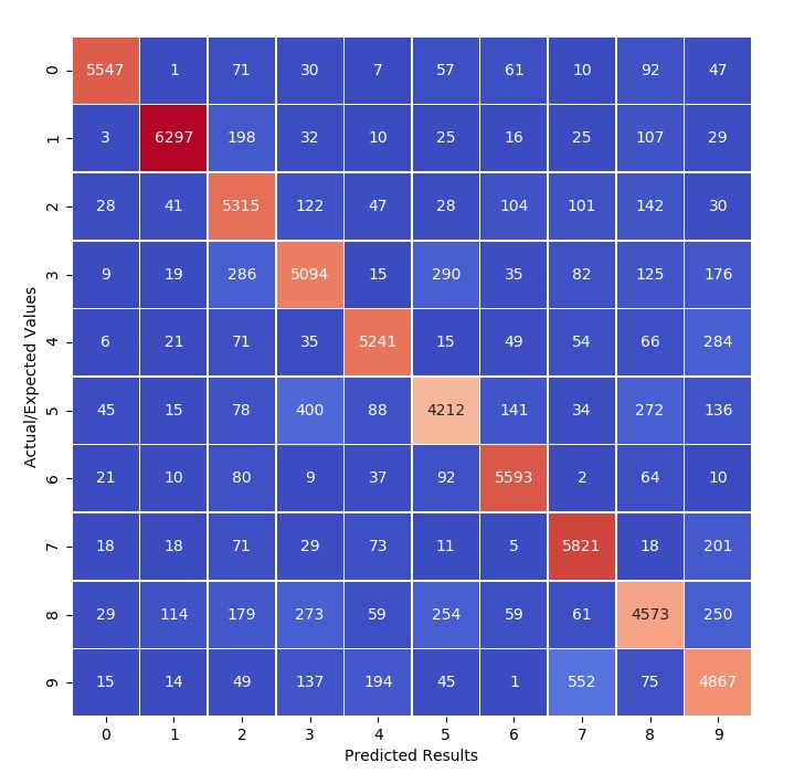
clf.fit (X_train, y_train)Instead of finding the precision, recall, and any ROC curves, a confusion matrix is instead used. The confusion matrix lists the number of predictions made for each actual value. In the ideal case, all results should be listed along the diagonal. Below is the code the is needed to produce the confusion matrix.
from sklearn.model_selection import cross_val_predict
from sklearn.metrics import confusion_matrix

y_train_pred = cross_val_predict (clf, X_train, y_train, cv=3)
conf_mx = confusion_matrix (y_train, y_train_pred)
To make things easier to understand, the heatmap tool can be used from the seaborn package to produce a more visually striking confusion matrix as seen below.
Normalizing the results by dividing each row by the row’s sum, then the incorrect classifications can stand out a bit more predominantly. Note that the diagonal was zeroed out to avoid any confusion.
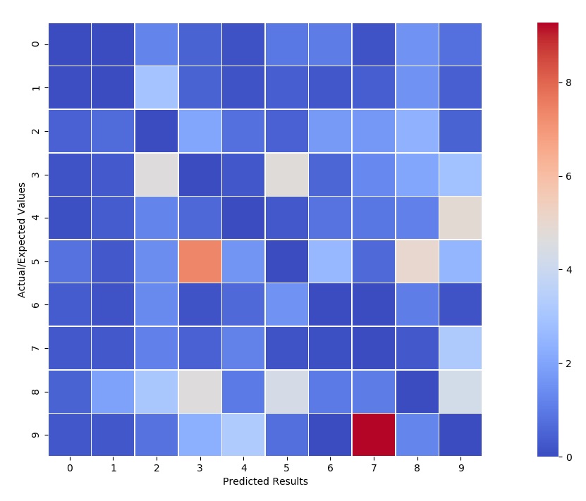
From the ‘normalized’ confusion matrix we see that a few cases are a bit more interesting to consider than others. These are all the non-blue squares. In the graph below the decision function results for each of the ‘cases of interest’ were shown.
Code…
All the code for this project, which include Javascript apps, Python code, and Jupyter notebooks is available here.
No Comments