First the overall goal should be mentioned… the aim create a model that will classify small images of clothing items. That is, by learning patterns from a set of 60,000 labelled training images, it is possible to predict the category from 10,000 unseen images.
The MNIST dataset is good as an introductory dataset, however there are some problems with it including (the following details were taken from here):
- MNIST is too easy. Convolutional nets can achieve 99.7% on MNIST. Classic machine learning algorithms can also achieve 97% easily. In some cases, pairs of MNIST digits can be distinguished by just one pixel.
- MNIST is overused. There are more interesting and complex datasets out there.
- MNIST can not represent modern CV tasks
Hence, some new datasets have been developed which can be considered as MNIST replacements/substitutes. Perhaps the most famous MNIST replacement is the Fashion-MNIST dataset where 10 categories of clothing are used instead of the digits 0 to 9. And just like MNIST, Fashion-MNIST has 70,000 28×28 grayscale images (60,000 for training and 10,000 for testing).
The categories in Fashion-MNIST include:
- T-shirt/top
- Trouser
- Pullover
- Dress
- Coat
- Sandal
- Shirt
- Sneaker
- Bag
- Ankle boot
Also some sample images from the dataset for all the categories can be seen below…
A few different neural network techniques were used to try to classify the dataset, including a simple dense network, two different convolutional neural networks, and two variations with the LeNet-5 network. It should be noted that there are a lot of other ‘popular’ networks out there but they weren’t used for a variety of reasons. The most relevant is that most of these networks (such as ResNet and VGG) are rather deep and can take a fair bit of time to compute on older computer that doesn’t have a GPU. For example, this VGG based network produced great results but required a lot of epochs to get there. Perhaps in the future this project will be revisited and the larger networks will be looked into.
Simple Dense Network
From previous work, some success was had with using a simple (dense) neural network with the MNIST dataset. Since there are some parallels between the MNIST and Fashion-MNIST, it seems like a logical choice to start things off from.
The following code was used to create the network, where three dense layers were used with the relu and softmax activation functions.
model = keras.Sequential ()
model.add (keras.layers.Flatten (input_shape=[28,28]))
model.add (keras.layers.Dense (units = 300, activation = 'relu'))
model.add (keras.layers.Dense (units = 100, activation = 'relu'))
model.add (keras.layers.Dense (units = 10, activation = 'softmax'))
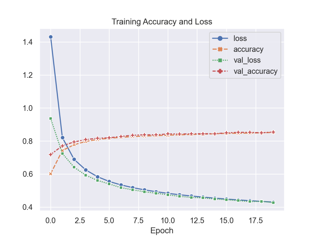
model.compile (optimizer = keras.optimizers.SGD(lr=1e-3), loss = 'sparse_categorical_crossentropy', metrics=['accuracy'])Since this network is pretty simple, training is pretty quick where an epoch takes less than 10s. After 5 epochs, the system starts converging (and begins to overfit) which results in an accuracy of 83.86% with the test set. Below is the accuracy and loss results obtained during training.
Convolutional Neural Network 1
Next, a convolutional neural network (CNN) similar to the previous MNIST project was used. This model contained 3 convolution layers (using 3×3 sized kernels), 2 max pooling layers, 1 standard output layer (using softmax for its activation function). Some of the code to build this model can be seen below:
model = keras.Sequential ()
model.add (keras.Input (shape=inputShape))
model.add (keras.layers.Conv2D (32, kernel_size=(3, 3), activation='relu'))
model.add (keras.layers.MaxPooling2D (pool_size=(2, 2)))
model.add (keras.layers.Conv2D (64, kernel_size=(3, 3), activation='relu'))
model.add (keras.layers.Conv2D (64, kernel_size=(3, 3), activation='relu'))
model.add (keras.layers.MaxPooling2D (pool_size=(2, 2)))
model.add (keras.layers.Flatten ())
model.add (keras.layers.Dropout (0.5))
model.add (keras.layers.Dense (10, activation='softmax'))
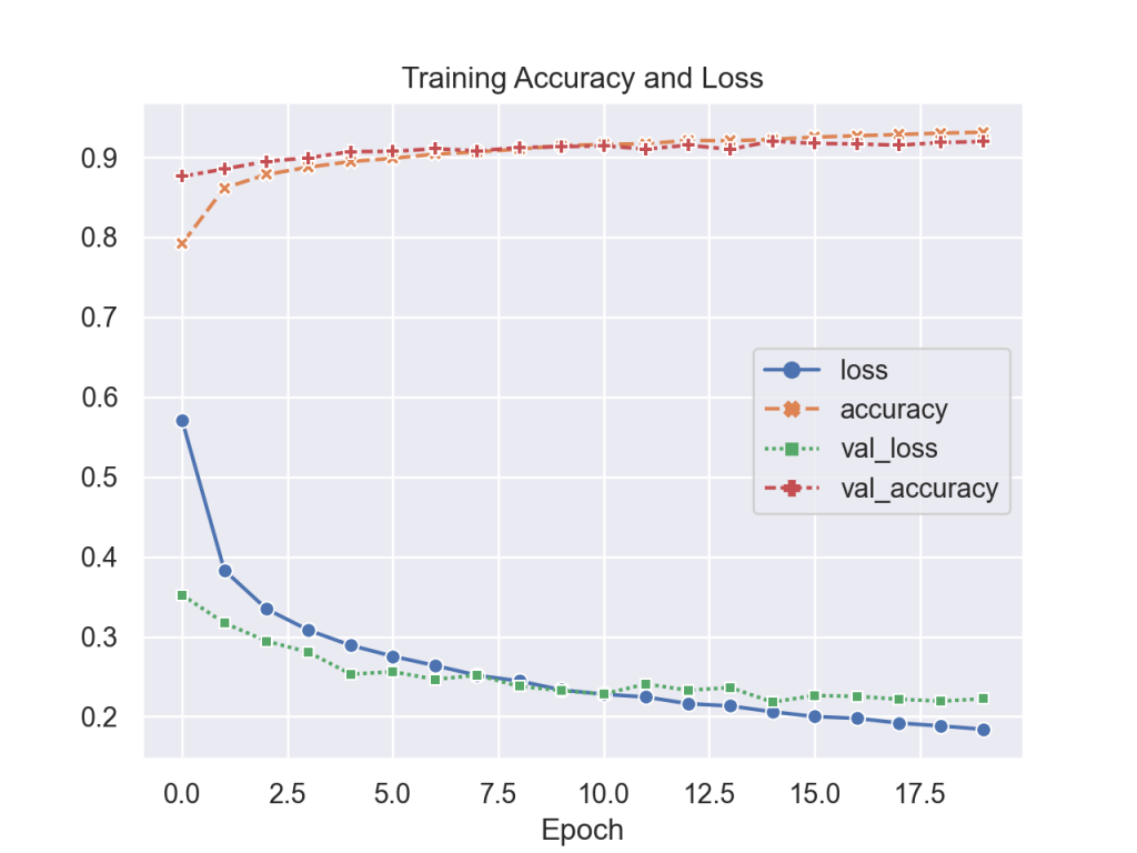
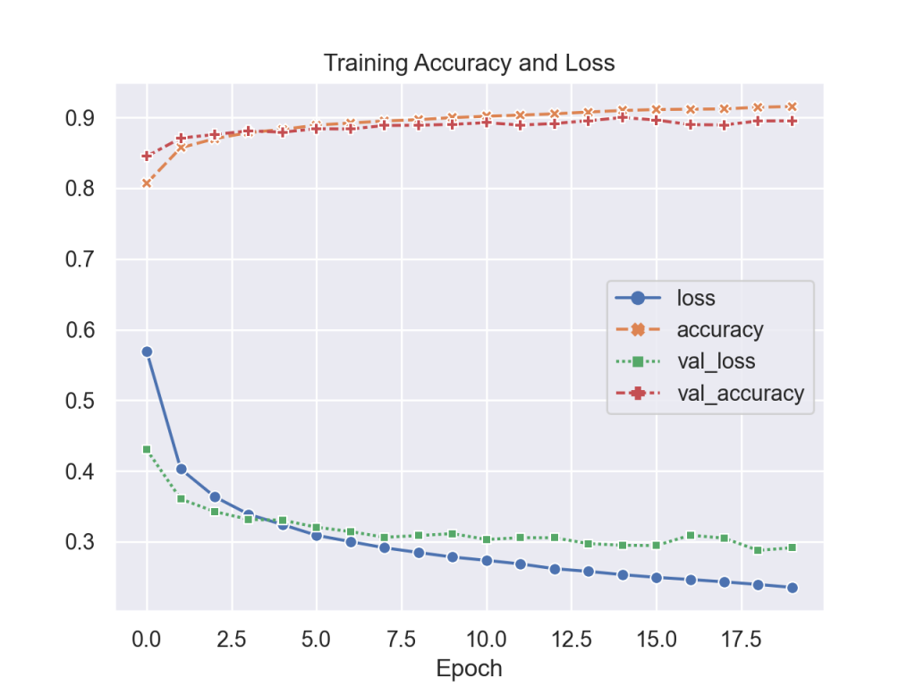
model.compile (optimizer = 'Nadam', loss = 'sparse_categorical_crossentropy', metrics=['accuracy'])Training this model takes longer with approximately 1 minute per epoch. However, accuracy is improved where a score of 91.6% was obtained with the test set. Also overfitting starts at around 8 epochs so the training process can be shortened.
Convolutional Neural Network 2
Next, more layers were added the previous CNN in an attempt to improve the accuracy. The main changes include adding more filters used for each convolution layer and more drop out layers. The code to build such a network is shown below:
model = keras.Sequential ()
model.add (keras.layers.Conv2D(32, (3, 3), padding='same', activation='relu', kernel_initializer='he_normal', input_shape=inputShape))
model.add (keras.layers.MaxPooling2D((2, 2)))
model.add (keras.layers.Dropout(0.2))
model.add (keras.layers.Conv2D(64, (3, 3), padding='same', activation='relu'))
model.add (keras.layers.MaxPooling2D((2, 2)))
model.add (keras.layers.Dropout(0.2))
model.add (keras.layers.Conv2D(128, (3, 3), padding='same', activation='relu'))
model.add (keras.layers.Dropout(0.5))
model.add (keras.layers.Flatten())
model.add (keras.layers.Dense(128, activation='relu'))
model.add (keras.layers.Dense(10, activation='softmax'))
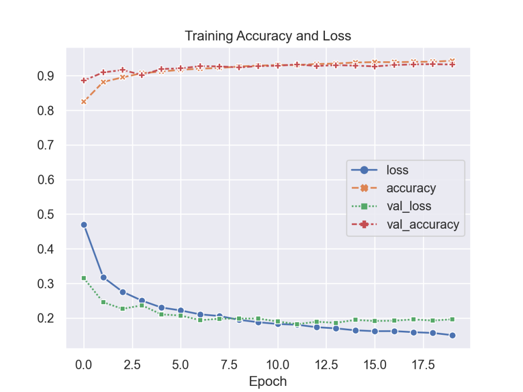
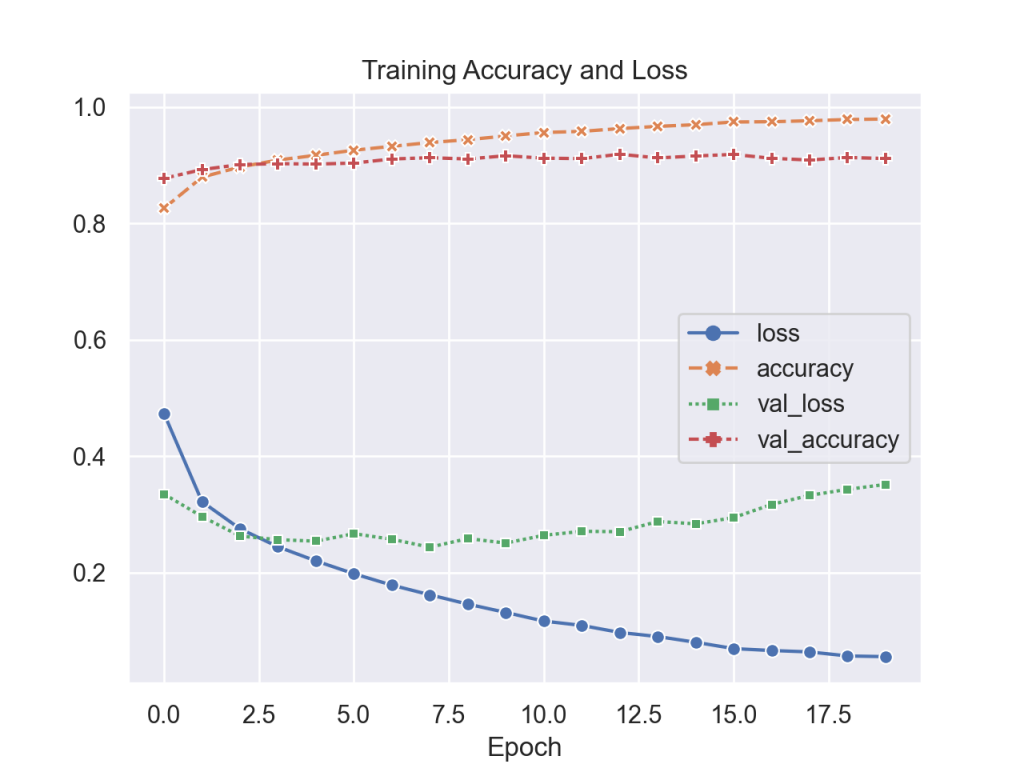
model.compile (optimizer = keras.optimizers.Adam (lr=0.001), loss = 'sparse_categorical_crossentropy', metrics=['accuracy'])Training takes a bit longer with each epoch taking approximately 85-90s, however accuracy improves to 92.9%. Also, only 8 epochs are needed since the model starts overfitting at that point.
LeNet 5
LeNet-5 is an early well known CNN that was originally designed to classify the MNIST dataset (some nice videos of some results can be seen here). It is a bit older, and hence uses some concepts that are not too popular anymore (such as tanh activation functions). From the original paper, the network can visually be described as:
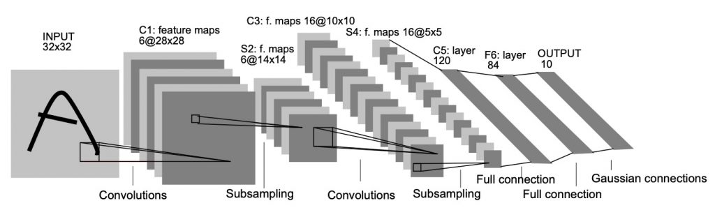
Some details about the layers include:
- The input uses 28×28 images that have been zero padded by 2 pixels which makes them 32×32 in size. This is so that the first convolution operation won’t reduce the size of the image.
- Instead of max pooling, average pooling was used. The original LeNet average pooling is slightly more complicated in that the computed value is multiplied by a learned weight and bias value.
- The tanh function was used as the activation function instead of the trusty relu function. It is a sigmoidal function that ranges from -1 to +1 with a mean value of 0.
- The final activation function (Radial Basis Function or RBF) is a bit different in that it squares values; this is good since it can help converge values more quickly.
Below is the code used to create this network:
model = keras.Sequential ()

model.add (keras.layers.Conv2D (6, (5,5), padding='same', activation=tf.nn.tanh, input_shape=(32, 32, 1)))
model.add (keras.layers.AveragePooling2D ((2, 2), strides=2))
model.add (keras.layers.Conv2D (16, (5,5), padding='same', activation=tf.nn.tanh)
model.add (keras.layers.AveragePooling2D ((2, 2), strides=2))
model.add (keras.layers.Conv2D (120, (5,5), activation=tf.nn.tanh))
model.add (keras.layers.Flatten ())
model.add (keras.layers.Dense(84, activation=tf.nn.tanh))
model.add (RBFLayer(10, 0.5))#keras.layers.Dense(10,  activation=tf.nn.softmax))

model.compile (optimizer = 'adam', loss = 'sparse_categorical_crossentropy', metrics=['accuracy'])
Training the system took close to 45 second per epoch achieved an accuracy of 88.9% with the test set (as seen below).
Modified LeNet 5
By changing a few critical elements from the previous LeNet CNN implementation, slightly better model accuracy can be achieved. The big changes are simply replacing the activation functions; that is relu for tanh and softmax for RBF. By doing so the accuracy improves to 90.6%.
Overall Results…
Below is a summary of the results.
| Network Type | Accuracy | Ave. Training Time per Epoch | Min Epochs |
| Simple NN | 83.86% | < 10 s | 5 |
| CNN 1 | 91.6% | ~60 s | 8 |
| CNN 2 | 92.93% | ~85 – 90 s | 8 |
| LeNet 1 | 88.89% | ~45 s | 3 |
| LeNet 2 | 90.55% | ~45 s | 3 |
Looking at the Results…
Below is an interactive confusion matrix showing some of the incorrectly classified results. The big things to notice include:
- There is some overlap between some of the fashion categories. For example, some shirts can be t-shirts/tops, pullovers, and perhaps even dresses. Also there is some confusion between sneakers and ankle boots.
- The amount of low level details in the Fashion MNIST dataset is much higher than with the regular MNIST dataset. Hence a 28×28 sized image may not capture all such details. If the images were larger, perhaps the accuracy would be somewhat improved.
- There are a few outliers in the data set that either should be removed before the model is determined, or more images of such items should be added so they aren’t outliers.
- Perhaps data augmentation should be performed to improve the accuracy of the model.
Code…
All the code in both Python (for the actual TensorFlow work) and Javascript (for the interactive web stuff on this page) is available here.
Some Interesting Notes…
While working on this project, I came across a few academic projects with this dataset. The overall goals with this for me was to have some fun while learning some new things; however for some people this dataset inspired papers to be published and even use it as a core element in a masters thesis.
No Comments