A little while ago I noticed a few posters in the office I used to work in had a bunch of graphs with the occasional presence of a bifurcation element amidst the plethora of information they presented. I tried to read and follow all of these posters but none of them lead to the reason why they were present. I had some cursory knowledge on the topic and felt I should do some research on my own to improve of what I know about them. Also, I felt it would be a good opportunity to ‘keep my programming sword sharp’ so I decided to write some code where I could explore bifurcation diagrams in four different languages.
This video is excellent in explaining some of the background on the subject (note that only some of them are explored in more detail below).
Background
Bifurcations can occur from a variety of conditions/functions and perhaps the most well known are the ones based on the ‘logistic equation’. Belgian mathematician P. F. Verhulst studied differential equations related to population growth rates which is what this logistic equation is based on.
One of the simpler models is based upon the population growth under ideal conditions (with a constant supply of food and space, and no predators). A few elements to keep the model simple are:
- The next generation is dependent on the results from the previous generation (that is the value of N_{n+1} is dependent on the value of N_{n})
- The capacity of the system is set to 1, so hence the results can be interpreted as a percentage (or mathematically 0 \leq N_{n} \leq 1)
- The growth rate is represented by one parameter, that is \mu
- The population grows when N_{n} is small since it can increase if since there is ample food and space. It declines when N_{n} is large since new generations need to compete for food and overcrowding.
Therefore the logistic equation is defined as:
The continuous version of the above equation (which is easier to study) is:
Note that the Q stands for quadratic.
To study the dynamics of the population growth, we repeatedly call the quadratic equation and analyze the results; that is we need to analyze the following sequence:
Note that Q_\mu^{n}(x_0) is the shorthand for the nth iteration of x_0 for Q with a constant \mu value. Also, the sequence can be written in the following shorthand notation: \left\{Q_\mu^{n}(x_0)\right\}^\infty_{n = 0}
When studying such iteration based sequences, a few different results commonly occur:
- It can diverge to infinity. We are not interested in such results, hence we put constraints on \mu and the initial value x_0
- It can converge to a certain value which is commonly called the fixed point. Note that there are attracting and repelling fixed points; with the function and conditions we are using we won’t worry about repelling fixed points. More details can be found here: Wikipedia, U of Toronto Math 335 notes, and U of Wisconsin chaos notes
- It can jump among a set n of values, which is commonly referred to as person-n point. The periodic orbit is often called an n-cycle.
- There can be no pattern; that is there is a chaotic solution.
With the quadratic function Q_\mu, there are some notable regions of interest when examining the iteration results. I am going to skip over some of the deeper math on why it occurs since that can be referenced from various online sources of even textbooks (like this one). Note that the different regions only depend on \mu and not at all on the starting value (x_0). Also to note, the number of iterations should be large, that is the eventual pattern doesn’t usually occur within the first few iterations. Hence, depending on the value of \mu, the iteration behaviour is as follows…
0 < \mu \leq 1
The sequence converges to 0; that is 0 is the systems fixed point
1 < \mu \leq 2
The system converges to one fixed point, that is 1 – 1/\mu. Note that there actually are two fixed points in the system, 0 is a repelling fixed point, and the noticed one is an attracting fixed point.
2 < \mu \leq 3
the system starts oscillating between certain solutions, but after a large number of iterations converges back to a fixed point (which is 1 – 1/\mu).
3 < \mu \leq 4
Things get interesting and complicated…
Over the range from 3 to 3.4494… (or more precisely, 3 < \mu \leq 1 + \sqrt{6}) values oscillate between two values; that is the results form a 2-cycle. Mathematically it can be shown that for values in the range \mu_{n-1} < \mu \leq \mu_n, then the solution has a 2^k-cycle for values of (k of 0, 1, 2, \ldots, n). These successive values of \mu can be computed by:
Note that \mu_k has a limit, that is \mu_\infty = 3.61547\cdots ; this value is where the bifurcation (or period doubling) points stop and where an unpredictable behaviour occurs.
The rate that the period doubling occurs can be calculated as:
Note that the letter d was chosen to indicate the distance between succeeding bifurcations. This value converges to a special constant called the Feigenbaum constant, which is named after Mitchel Feigenbaum (another great Feigenbaum article) who originally discovered it, and is:
This value is a universal constant, since other ‘one-humped’ functions result in the in the same value.
The following tool can be used to experiment with seeing how Q_\mu^{n}(x_0) takes on different values for \mu (click here to view it in a separate tab).
Bifurcation Diagrams
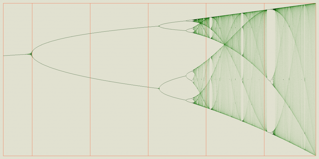
A bifurcation diagram is a 2d graph where the horizontal axis corresponds to various values of \mu and the vertical axis represents the various values of the resulting fixed points. It is fractal in nature since it has self similarity; also it can be zoomed in countless numbers of times to reveal more details.
For a single \mu value it is possible to determine fixed points by hand using a calculator. However, for the complete set of \mu values it is quite difficult. Hence, to be efficient it is best to write some code.
Implementations…
A few different implementations were created to produce bifurcation diagrams. These include:
- Python: mainly to keep my python skills sharp, and also perhaps it is the easiest language to deal with. Also to experiment a bit with interacting with graphics files.
- Javascript: I feel one needs to be able to make both stand alone apps and web based apps nowadays. So this was some practice with that.
- C# .Net Console based: I am trying to get a little deeper and improve my C# programming. This was to try out a few things to try to make a more minimal command line based application.
- C# .Net WinForms based: Another attempt on using C# to make a minimal windows based application
Main Algorithm
The main algorithm is quite simple and based on the following psuedo-code listed below:
for mu = muMin to muMax by muStep
    x = 0.5
    for i = 1 to maxIterations
        x = mu * x * (1 - x)
        if i > minIterations
           plotPixel at (mu, x)
Note that the minIterations variable is used to not account for any initial iterations since we are only concerned with the ‘eventual’ fixed points not the initial values. Also, to make the resulting diagram a little more visually appealing, the resulting fixed points are shaded by the frequency of their occurrences.
All code is available in the following GitHub repository.
Python Implementation
The python version was implemented first since it was perhaps the easiest language to deal with. All image handling was done using the PIL package. Note that the background image at the top of this page was created using this implementation.
Javascript Implementation
To try to be a bit more efficient, a fast pixel handling technique was used so that the calculation was done once and then written to the canvas one time. More information about this technique is available here.
To be nice and take less resources since the calculations are performed on the clients machine, a ‘compute’ button was added so that the computation is performed selectively instead of far too often. Click here to view it in a separate window.
C# .Net Console Implementation
Next a Windows console app using C# .Net Core was used. The overall implementation is rather similar to the Python one in where the computation results are written to an image (or Bitmap) and then the image is written to a file (as a jpeg).
One item to note is that some additional setup needs to be performed in order for the code to compile/link correctly. Using the ‘Manage NuGet Packages…’ (accessed by right clicking on the project in the Solution Explorer), the ‘System.Drawing.Common’ tool needs to be installed first before anything is built.
One additional feature was added to allow for some vertical lines to be drawn at specific values of \mu. Note that the one major benefit of this and the python versions is that a much higher resolution image can be generated since we are not dependent on screen resolution.
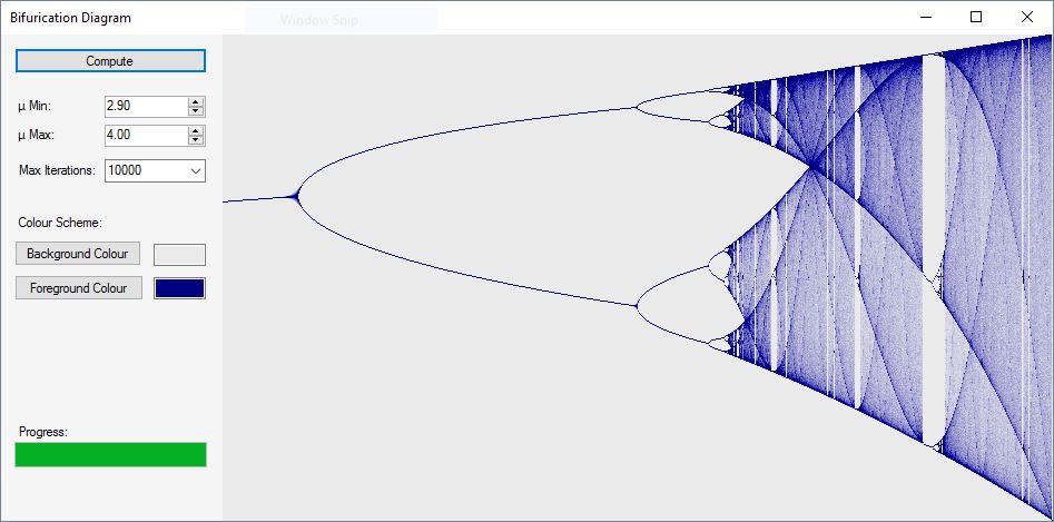
C# .Net WinForms Implementation
Finally, a C# .Net Windows Forms application was created so that a more traditional GUI based tool was used. The graphics were mainly accomplished using the GDI+ library. Also, in a similar manor to the previous console application, the calculations are written to a bitmap, and then displayed to the screen by acquiring a panel’s graphics object and then calling the drawImage image object. The main idea why the graphics update was performed this way was that it was rather quick since it was called often by the paint event.
While this version is similar to the Javascript version, two small changes were introduced since they are readily available with Windows. These are colour picking dialogs (to choose the background and foreground colours) and updating a progress bar when computing the results.
No Comments