With the current Covid-19 pandemic, there has been some talk about virus propagation in the media. It seems that there is a lot missing among the various news sources. I find that their explanations to either be not technical enough or just missing a lot of key details. Also, I expect that certain types of web content to be interactive and slightly engaging. Therefore in my spare time I have decided to make a small set of Covid-19 projects to make sense of some of the data and information for myself.
There are multiple ways to simulate virus propagation. Perhaps they can be placed into two categories: numeric (bouncing balls or grid based) or using differential equations. Both numeric and differential equation based techniques will be briefly examined with this project. To start off, the numeric bouncing ball model was made to have some simple visual demos to show how a virus can propagate within a population.
Note that the demos are purely for a ‘visual explanation’ of the process of how a virus can propagate through a population. There are a few issues with drawing some serious conclusions from it. First and perhaps most obvious is that people can not be represented by little balls within a box, since most people have free will and usually do what they do. Secondly, if any serious conclusions could be drawn from the simulations, a large amount of simulations need to be done over many variations of variables need to be done; at that point the simulations would need to be purely numerical.
Bouncing Ball Virus Model
The bouncing ball model assumes that the virus (or virus carrier or person) is a ball on a 2D plane that bounces around in a closed space that contains other balls. The virus is transferred when an infected ball hits a non-infected ball. Each bounce follows the basic billiard ball collisions; that is the angle of reflection is equal but opposite to the angle of incidence.
Also to keep things simple, the initial state of the simulation is determined purely at random. That is, the ball positions are chosen at random so that none at coincident and the directions are all randomly chosen as well. The initial speeds are specified by the user.
Basic Physics
The physics for this simulation assume that there are no external forces such as gravity or friction, also both kinetic energy and momentum are conserved, and all collisions are 100% elastic.
Since we are dealing with elastic collisions, then the momentum (p) doesn’t change, that is \Delta p = 0. So mathematically we have:
Also, we are assuming that the kinetic energy is conserved in the system. Therefore we have:
Combining these two relationships, then in an one dimensional case the velocities can be calculated by the following:
In a two dimensional case, the calculations are slightly more involved. First the line of collision between the two balls must be determined using the balls’ center points. Then the vector components of the balls’ velocities are found with respect to the line of collision. Velocities tangent to the point of collision do not change while the ones that run in the same direction can be calculated using the above equation. The mathematics can be efficiently written as:
Where \langle \cdot \rangle is the dot product, and x_1, x_2 are each ball’s center points.
Simplest Case
In the simplest case, an infected ball interacts with those that have not been infected yet. Since the options are rather limited, this case can be used to see the general trend of how a virus can propagate.
The user is able to change the following parameters:
- Initial Speed: The speed of the balls set at the beginning of the simulation. To keep things simple, a few qualitative values were chosen so that the simulation performs reasonably ok
- Total Population: The total number of balls in the simulation (or box). For now only a few different settings are possible, including: 25, 50, 100, 200, and 400 balls.
- Initial Infections: The number of infections at the start of the simulation. To keep things simple only 1, 2, 5, and 10 infections are possible.
- Infection Rate: The probability that an infection will occur during a collision. For example, an infection rate of 75% means that an infection has a random chance of occuring 3 out of 4 times per collision. Note that this value is purely qualitative and does not correspond to the R_0 value.
Note that the above demo is can be viewed in a separate window here.
Results
The simulation is fairly simple, it does show that social distancing does slow down the transmission of the virus. This can be be seen by adjusting the number of balls; more balls results in less time for all the balls to be infected.
Also, the results show that the infection rate impacts how long before all the balls are infected. It should be noted that different virus have different infection rates so this feature can be used to compare the behaviour of different viruses. Also, one can argue that wearing various personal protective equipment (such as masks), can also reduce the infection rate as well.
Case 2: Dealing with States
To make the simulation slightly more realistic, the virus propagation can take the following states:
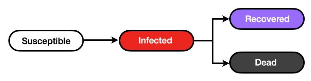
Where:
- Susceptible represent the those who have never had the virus. They can only be infected.
- Infected are those who have the virus, that is they have been infected. They can infect those who are susceptible. Also, those who are infected will move to the next states by a user specified time.
- Recovered represents those who no longer are infectious and can not transmit the virus to others. It is assumed that they are immune to future infections.
- Dead are those who have died by the virus. Again, it is assumed that they do not transmit the virus either. Also, the dead no longer move but can if hit by another ball.
The demo is based upon the previous simulation where a few more features have been added to it, namely:
- Infection Time: is the time for those in the infected state. This ‘time’ is based on the number of moves rather than an actual time.
- Death Rate: is the probability that someone will die after they have been infected. A value of zero represents no deaths will occur, while 100 results in all
Note that the above demo is can be viewed in a separate window here.
Results
Here the main element to notice is that shorter infection times and low death rates, can result in a many susceptible people to not to get infected. This is due to those who are recovered are immune and can ‘block’ those who are susceptible from getting infected.
Case 3: States and Vaccination
An additional state was added to account for those who have been vaccinated. Therefore, the initial population can be either susceptible or vaccinated. Also, note that it is possible to adjust the effectiveness of the vaccine so that it is still possible for someone to be still infected by the virus.

This case’s demo is built upon the previous case and a few additional features were added on to it, which include:
- Initial Vaccinations: accounts for the initial number of people (or balls) that have received a vaccine.
- Vaccine Effectiveness: allows one to specify how effective a vaccine is. It should be noted that most vaccines are far from being 100% effective. Also, the efficacy can vary depending on many factors including age of the population and the severity of the infection (hospitalization, death).
Note that the above demo is can be viewed in a separate window here.
Results
By vaccinating a good amount of the population (at least 60%) with a highly effective vaccine (90+%), then it is possible to have a very small amount of of virus propagation, and so a small amount of the susceptible population will get infected.
Overall…
While all of these demo simulations are fairly primitive, they show that social distancing, wearing PPE, and vaccination really can reduce the spread of a virus.
Code…
All code for the above demos is available here. Note that they were written in javascript and graphics were done using HTML5’s canvas tag.
No Comments