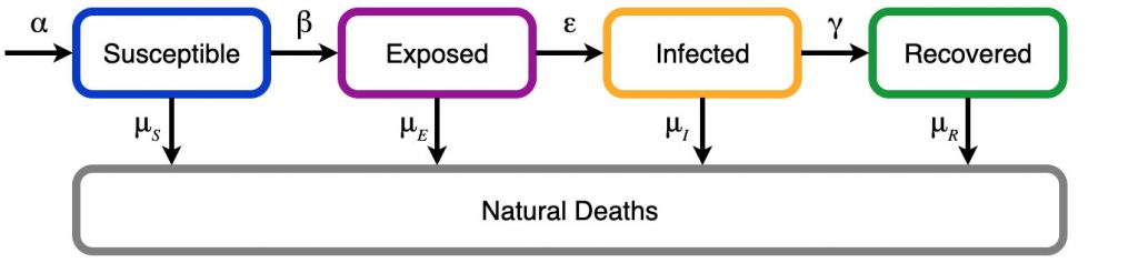
The SIR Model is a little basic and does not model Covid-19 very well. The SEIR model introduces extra parameters that can make the modelling a bit more accurate. The main change is the introduction of a new ‘exposed’ compartment, so we now have Susceptible, Exposed, Infected, and Recovered (or removed) compartments:

There is a fair bit of variation in the implementation of this model. Most implementations consider births at the susceptible level and naturally occurring deaths at all levels. Other models consider vaccination which allow susceptibles to go directly to the recovered/removed stage, partial immunity which results in recovered individuals returning back to the susceptible state, and asymptomatic recovery where exposed individuals skip the infected state. For our model we only consider births (\alpha) and natural deaths (the \mu‘s), that is:
Model Equations
Since this is a compartmental model equations are quite easy to determine (again please refer to the SIR Model document for more information on the compartmental modelling):
Where the model variables are:
- S are the susceptible individuals and are affected by the number of incoming individuals (\alpha), infected individuals, and the any resulting from natural deaths
- E are the exposed individuals. These account for any asymptomatic individuals (have been infected but are not showing any symptoms yet).
- I are in infected individuals.
- R are the recovered or removed individuals. This includes both those that have fully recovered (and are immune) and any deaths.
And the model parameters are:
- \alpha – Birth rate: this can be combined with any increase to the susceptible population, that is migration, immigration, and of course births.
- \beta – Transmission rate: is the infection rate, or how often a susceptible individual is in contact with an infected member results in a new infection (is the same as in the SIR model).
- \epsilon – Exposed to infected rate. This is used to account for the rate of asymptomatic/exposed individuals to become fully infected.
- \gamma – is the recovery rate, or how quickly an infected individual recovers (again is the same as the SIR model).
- \mu – is the natural death rate. Note for simplicity it will be the same for all of the compartments.
Please refer to this video by the tutor wizard for more details about the math behind the model equations.
Model Visualization
Since these are coupled non-linear differential equations, the solution can only be determined numerically using the same technique as the SIR model was previously. The following is interactive D3 based visualization of the ODE solutions.
For those who can not deal with the margins that wordpress puts onto page content, a full window version is available here.
Some things to note:
- This visualization is purely qualitative and is to aid in the understanding of the SEIR model. If one finds it useful that is great, however do not use it to make any predictions
- To keep things simple, the initial values were normalized, that is S + E + I + R = 1
- The initial values that were used are S_0 = 0.99, E_0 = 0.01, and I_0, R_0 = 0
Code…
The code for this visualization along with a Jupyter notebook is available to download at GitHub
Determining R0
For completeness, the basic reproduction number or R_0 can also be computed. It can be considered the expected number of new/secondary cases produced by a single (average) infection in a susceptible population. Instead of having a math heavy document, using the following set of slides (from the Workshop on Mathematical Models of Climate Variability, Environmental Change and Infectious Diseases) as a reference, we can determine R_0 to be:
No Comments