This problem is fairly simple to describe… given a bunch of variables that describe the various aspects of a house along with a sales price, is it possible to come up with a mathematical model that can be used to predict future prices based on different values of the same variables? It is based housing sales data from Ames Iowa between the years 2006 – 2010. (I am not sure if it work for Toronto sales data where its common to get huge sold over asking amounts which would make it difficult to predict sales prices).
If I had taken any econometrics courses, I would have learned that this problem can be considered as a Hedonic pricing model; from Investopedia:
Hedonic pricing is a model that identifies price factors according to the premise that price is determined both by internal characteristics of the good being sold and the external factors affecting it.
In finding a suitable model, there are few issues to deal with, including:
- There are 79 features which may be more than necessary; that is some features may provide more value than others when making a prediction
- How to deal with missing values? Drop them or fill them in with something reasonable (what is reasonable)
- How to deal with outliers?
- How to treat categorical data? What type of encoding should be used
Features…
Again, there are 79 features the dataset. Below is a brief description of them all (taken from the data dictionary with a few added notes):
- MSSubClass: Categorical variable that identifies the type of dwelling involved in the sale. An example value is 60 which refers to a ‘2-Story 1946 & Newer’ house
- MSZoning: Identifies the general zoning classification of the sale. Another categorical variable; ex. ‘RL’ refers to ‘Residential Low Density’
- LotFrontage: Linear feet of street connected to property
- LotArea: Lot size in square feet
- Street: Type of road access to property. Categorical variable with two values: ‘Grvl’ and ‘Pave’ for Gravel and Paved
- Alley: Type of alley access to property. Categorical variable with three values: ‘Grvl’, ‘Pave’, and NA for Gravel, Paved, and No Alley access
- LotShape: General shape of property. Categorical with options for regular to various shades of irregular
- LandContour: Flatness of the property. Another categorical variable with options for level, banked, hillside, or depression
- Utilities: Type of utilities available. Either all, all with no sewer, all with no sewer and water, or only electricity
- LotConfig: Lot configuration. Categorical describing where on the street the house is located; for ex. corner lot
- LandSlope: Slope of property. Categorical; ex. moderate slope
- Neighborhood: Physical locations within Ames city limits. String with up to 7 letters indicating the neighbourhood name. Note that ‘Names’ corresponds to North Ames
- Condition1: Proximity to various conditions such as adjacent to a major street, railroad, or park. Again categorical
- Condition2: Proximity to various conditions if more than one is present
- BldgType: Type of dwelling. Choices are in 5 categories including: single family detacted, two-family conversion, duplex, townhouse end unit, and townhouse inside unit
- HouseStyle: Style of dwelling. Eight categories including one story, two story, and split level
- OverallQual: Rates the overall material and finish of the house. Ranges from 1 for very poor to 10 for very excellent
- OverallCond: Rates the overall condition of the house. Same range as above, that is 1 for very poor to 10 for very excellent
- YearBuilt: Original construction date
- YearRemodAdd: Remodel date (same as construction date if no remodeling or additions)
- RoofStyle: Type of roof. Categorical with the following options: Flat, Gable, Gabrel, Hip, Mansard, Shed
- RoofMatl: Roof material. Categorical with eight options: Clay tile, Standard shingle, Membrane, Metal, Roll, Gravel & Tar, Wood shakes, and Wood Shingles
- Exterior1st: Exterior covering on house. Categorical with 17 options; some include: Brick face, Stone, Stucco, and Wood Shingles.
- Exterior2nd: Exterior covering on house if more than one material is present. Same options as those listed above.
- MasVnrType: Masonry veneer type. Categorical with 5 options: Brick common, brick face, cinder block, none, and stone
- MasVnrArea: Masonry veneer area in square feet
- ExterQual: Evaluates the quality of the material on the exterior. Five options from poor to excellent.
- ExterCond: Evaluates the present condition of the material on the exterior. Again, five options from poor to excellent.
- Foundation: Type of foundation. Categorical variable with options such as Cinder block, poured concrete, and slab
- BsmtQual: Evaluates the height of the basement. The height of the basement has been grouped into five bins, along with one for no basement.
- BsmtCond: Evaluates the general condition of the basement. Again 5 categories to describe the condition (from excellent to poor) along with 1 for no basement.
- BsmtExposure: Refers to walkout or garden level walls. Categorical with 4 options along with 1 for No basement
- BsmtFinType1: Rating of basement finished area. Seven categories… 5 for quality of living quarters (from good to low quality), 1 for unfinished, and 1 for no basement.
- BsmtFinSF1: Type 1 finished square feet
- BsmtFinType2: Rating of basement finished area (if multiple types). Same categories as those listed above.
- BsmtFinSF2: Type 2 finished square feet
- BsmtUnfSF: Unfinished square feet of basement area
- TotalBsmtSF: Total square feet of basement area
- Heating: Type of heating. Categorical with 6 options including floor furnace and gas forced warm air furnace among others
- HeatingQC: Heating quality and condition. Five options from poor to excellent
- CentralAir: Central air conditioning. Either yes or no
- Electrical: Electrical system. Five options including: standard circuit breakers & romex, fuse box over 60 amp and all romex wiring, 60 amp fuse box and mostly romex wiring, 60 amp fuse box and mostly knob and tube wiring, and mixed
- 1stFlrSF: First Floor square feet
- 2ndFlrSF: Second floor square feet
- LowQualFinSF: Low quality finished square feet (all floors)
- GrLivArea: Above grade (ground) living area square feet
- BsmtFullBath: Basement full bathrooms. Integer value
- BsmtHalfBath: Basement half bathrooms. Again value is an integer
- FullBath: Full bathrooms above grade
- HalfBath: Half baths above grade
- Bedroom: Bedrooms above grade (does NOT include basement bedrooms)
- Kitchen: Kitchens above grade
- KitchenQual: Kitchen quality. Five options including: excellent, good, average, fair, and poor.
- TotRmsAbvGrd: Total rooms above grade (does not include bathrooms)
- Functional: How functional the home is (assume typical unless deductions are warranted). Options include minor deductions, moderate deductions, major deductions, severely damaged, and salvage only
- Fireplaces: Number of fireplaces
- FireplaceQu: Fireplace quality. Five levels of quality (from excellent to poor), and one option for no fireplace
- GarageType: Garage location. Options include: attached to home, basement garage, built-in, car port, detacted from home, more than one type, and no garage
- GarageYrBlt: Year garage was built
- GarageFinish: Interior finish of the garage. Options include: funished, rough finished, unfinished, and no garage
- GarageCars: Size of garage in car capacity
- GarageArea: Size of garage in square feet. Highly correlated with the garage cars feature
- GarageQual: Garage quality. Five options for quality (from excellent to poor), and one option for no garage
- GarageCond: Garage condition. Five options for condition (from excellent to poor), and one option for no garage
- PavedDrive: Paved driveway. Three options: paved, partial pavement, and dirt/gravel
- WoodDeckSF: Wood deck area in square feet
- OpenPorchSF: Open porch area in square feet
- EnclosedPorch: Enclosed porch area in square feet
- 3SsnPorch: Three season porch area in square feet
- ScreenPorch: Screen porch area in square feet
- PoolArea: Pool area in square feet
- PoolQC: Pool quality. Four options for condition (from excellent to fair), and one option for no pool
- Fence: Fence quality. Five options including: good privacy, minimum privacy, good wood, minimum wood/wire, and no fence
- MiscFeature: Miscellaneous feature not covered in other categories. These include: elevator, second garage, shed, tennis court, other, and none
- MiscVal: Dollar value of miscellaneous feature
- MoSold: Month Sold (MM)
- YrSold: Year Sold (YYYY)
- SaleType: Type of sale. Ten options including: warranty deed – conventional, warranty deed – cash, warranty deed – va loan, home just constructed and sold, court officer deed/estate, contract 15% down payment regular terms, contract low down payment and low interest, contract low interest, contract low down, and other
- SaleCondition: Condition of sale. Siz options including: normal sale, abnormal sale (such as a trade or foreclosure), allocation (two linked properties), family (sale between family members), and partial (home was not yet finished)
Data Cleanup
Overall to clean up the data after the NAs were dealt with, a combination of of the following options were performed (such as dropping features, outliers, and creating new features)
Dealing with NAs
First and foremost, we should check to see if any null values exist and what exactly to do with them.
Recall that one way to list the number of NAs for a feature within a dataframe is:
NumberNAs = DF[<Feature>].isna().sum()Using the above code, there are a total of 13965 NAs in the training set…
  MSZoning      -->     4   Categorical
  LotFrontage   -->   486   Numerical
  Alley         -->  2721   Categorical
  Utilities     -->     2   Categorical
  Exterior1st   -->     1   Categorical
  Exterior2nd   -->     1   Categorical
  MasVnrType    -->    24   Categorical
  MasVnrArea    -->    23   Numerical
  BsmtQual      -->    81   Categorical
  BsmtCond      -->    82   Categorical
  BsmtExposure  -->    82   Categorical
  BsmtFinType1  -->    79   Categorical
  BsmtFinSF1    -->     1   Numerical
  BsmtFinType2  -->    80   Categorical
  BsmtFinSF2    -->     1   Numerical
  BsmtUnfSF     -->     1   Numerical
  TotalBsmtSF   -->     1   Numerical
  Electrical    -->     1   Categorical
  BsmtFullBath  -->     2   Numerical
  BsmtHalfBath  -->     2   Numerical
  KitchenQual   -->     1   Categorical
  Functional    -->     2   Categorical
  FireplaceQu   -->  1420   Categorical
  GarageType    -->   157   Categorical
  GarageYrBlt   -->   159   Numerical
  GarageFinish  -->   159   Categorical
  GarageCars    -->     1   Numerical
  GarageArea    -->     1   Numerical
  GarageQual    -->   159   Categorical
  GarageCond    -->   159   Categorical
  PoolQC        -->  2909   Categorical
  Fence         -->  2348   Categorical
  MiscFeature   -->  2814   Categorical
  SaleType      -->     1   Categorical
Going through each of these features is a rather painful process (and was done in a separate Juptyer notebook). From that exploration, a few items were noticed:
- For some features NAs refer to None. So for Alley, FireplaceQu, GarageType, GarageFinish, GarageQual, GarageCond, PoolQC, Fence, and MiscFeature all NAs were replace with the string ‘None’
- For most categorical features the most frequently occurring value was used for the NA replacement. This was the case for: MSZoning, Utilities, Exterior1st, Exterior2nd, MasVnrType, BsmtQual, BsmtCond, BsmtExposure, BsmtFinType2, Electrical, KitchenQual, GarageCars, and SaleType
- Depending on the condition of the data, either the mean, median, or the mode were used for: LotFrontage, MasVnrArea, TotalBsmtSF, and GarageYrBlt
- For certain features the values were almost distributed between two or three options. For such cases a function was written to randomly select from the most commonly distributed using the frequency that they occur
- Some features are dependent on others and in such cases, some code was written to use the mean value based on the parent feature. This included: BsmtFinType1, BsmtFinType2, BsmtFullBath, BsmtHalfBath, and GarageArea
- And finally, BsmtUnfSF was calculated using the means or TotalBsmtSF, BsmtFinSF1, and BsmtFinSF2
Checking Feature Variation
Some features were almost entirely constant. Hence, there would provide very little information in the pricing model so they were very good candidates to be dropped. The following is a list of features and the percentages of how often a one value is used:
  Street           0.99588900
  Alley            0.93216855
  Utilities        0.99965742
  LandSlope        0.95169579
  Condition2       0.98972251
  RoofMatl         0.98526893
  BsmtCond         0.92086331
  Heating          0.98458376
  CentralAir       0.93285372
  Electrical       0.91538198
  LowQualFinSF     0.98629668
  BsmtHalfBath     0.93970538
  KitchenAbvGr     0.95409387
  Functional       0.93148338
  GarageCond       0.90921548
  PavedDrive       0.90476190
  3SsnPorch        0.98732443
  ScreenPorch      0.91229873
  PoolArea         0.99554642
  PoolQC           0.99657417
  MiscFeature      0.96402878
  MiscVal          0.96471394
As one can see Utilities, Street, Condition2, Heating, 3SsnPorch, PoorArea, and PoolQC are dominated by one value are are good candidates to be dropped.
Checking the Correlation to the Sales Price
Some features have little impact on the sales price and hence can possibly be dropped. It is easiest to see these using a heat map where the correlation is calculated between all the numeric values as seen below.
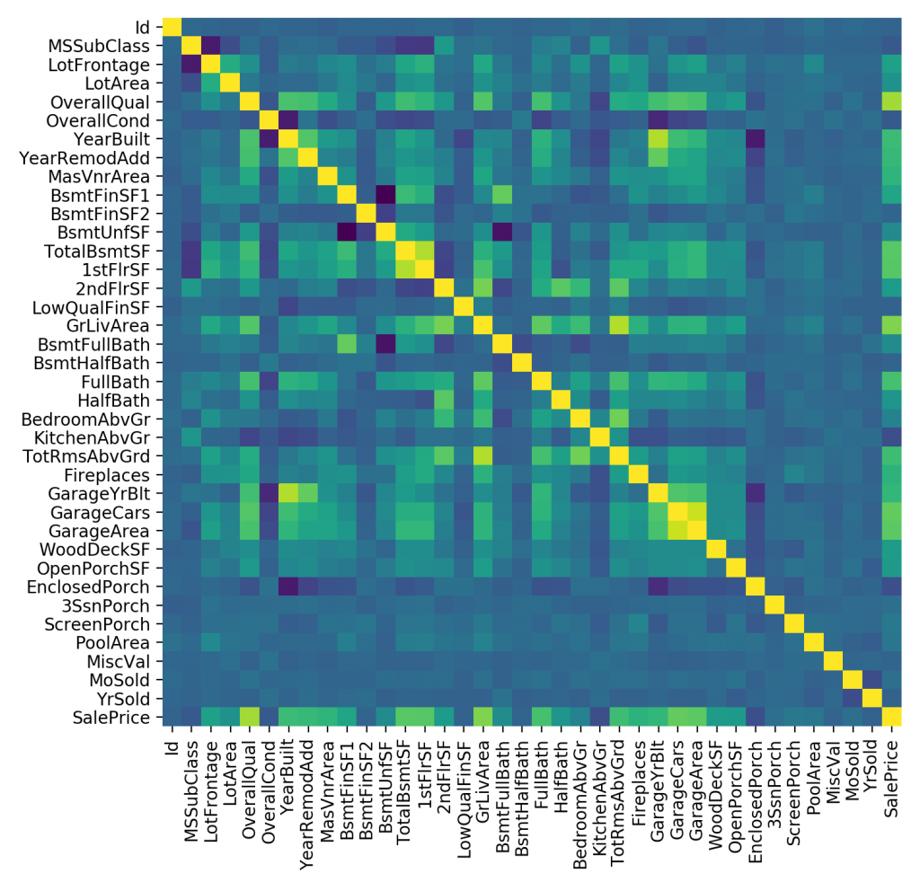
From the heat map, the main item of interest is which values have the greatest correspondence with the SalePrice. Considering both positive and negative correlation the features that have the least correlation with the SalePrice are: MSSubClass, LotArea, OverallCond, BsmtFinSF2, BsmtUnfSF, 2ndFlrSF, LowQualFinSF, BsmtFullBath, BsmtHalfBath, HalfBath, BedroomAbvGr, KitchenAbvGr, WoodDeckSF, OpenPorchSF, EnclosedPorch, 3SsnPorch, ScreenPorch, PoolArea, MiscVal, MoSold, and YrSold. All of these features are possible candidates that can be dropped.
Feature Engineering
It is possible to create new features from existing ones that will have more correlation with the sales price and then produce a better model. Some of the created features included the square feet per room (SqFtPerRoom), overall condition/quality, total number of baths, and the square feet above grade. Mathematically they were calculated using:
DF['SqFtPerRoom'] = DF['GrLivArea'] / (DF['TotRmsAbvGrd'] +
                                           DF['FullBath'] +
                                           DF['HalfBath'] +
                                           DF['KitchenAbvGr'] )

DF['OverallCondQual'] = DF['OverallQual'] * DF['OverallCond']

DF['TotalBaths'] = ( DF['FullBath'] +
                     DF['BsmtFullBath'] +
                     (0.5 * DF['HalfBath']) +
                     (0.5 * DF['BsmtHalfBath']) )

DF['AboveGradeSF'] = DF['1stFlrSF'] + DF['2ndFlrSF']
Note that an option made it possible to drop the features that were used with the new engineered feature (that is the dependencies).
Categorical Variable Encoding
Approximately half of the features are categorical and in order to effectively deal with them, they need to be label or one-hot encoded. An option was made so that during hyperparameter tuning, either method could be used and evaluated.
Dropping Outliers
Certain numerical features contained some extreme outliers. Our definition of an outlier was basically those values that were more than two standard deviations away from the mean. Note that during hyperparameter tuning it was possible to adjust if outliers should be dropped along with the number of standard deviations to use.
Scaling the Data
Since a few different models were used, therefore it was possible to scale the data using either the min/max or standard scaling, along with no scaling at all. Again, this option was able to adjusted during hyperparameter tuning.
Taking the Log of SalePrice
The sale price is somewhat skewed. One way to deal with this problem is to take the log of the price before it is fit to a model, then use the exponential function after a prediction is made. Note that this option is user controllable so that the quality of the results can be tested with logs both taken and not.
Models
A variety of models were used with the hope that one of them would generalize best to the data.
Recall that a linear model can be written mathematically as:\ell = \beta_0\ +\ \beta_1x_1\ +\ \beta_2x_2\ +\ \cdots\ +\ \beta_nx_n
Where \beta_0 in the intercept (or bias) and \beta_i (where 1 \leq i \leq n) is the weight (or slope) that controls the amount of a particular feature that is used.
One of the most common ways to prevent overfitting is to use some type of regularization, with the most popular are L1 (or ridge), L2 (or lasso), and elastic net (which is a combination of L1 and L2).
By using many combinations of data and model parameters, it was determined that the following parameters produced a model with best results:
- Ridge regression
- One-hot encoding
- No scaling
- Take log of sales price
- Drop feature with little variation
- Keep features with little correlation to the sales price
- Do not make new features,
- Drop outliers
Also this model obtained a kaggle score of 0.13574
Random Forest
The random forest algorithm uses multiple decision trees that are grouped together to commonly solve classification and regression problems. The grouping is commonly called ensemble learning.
During training both the data parameters (listed above) and model parameters were adjusted to produce a model that made the best predictions on a validation set (using cross fold validation). The model parameters that were adjusted included:
- Number of estimators. Possible values included: 200, 400, 600, 800, 1000
- Maximum number of levels in tree. Possible values included: 10, 20, 30, 40, 50, 60, 70, 80, 90, 100, 110, 120, 130, or none for max depth until all leaves are ‘pure’
- Minimum number of samples required to split a node. Possible values included: 2, 5, 10, 15
- Minimum number of samples required at each leaf node. Possible values: 1, 2, 4, 8, 16
- Bootstrap… whether bootstrap samples are used when building trees. If false, the whole dataset is used to build the tree (taken from SKLearn documentation)
During training the following combination of model and data parameters were found to produce a good fitting model (via cross fold verification):
- Label encoding
- Standard scaling
- Take log of sale prices
- Keep features with little variation or little correlation the sales price
- Do not make any new features
- Drop outliers
- Number of estimators: 1000
- Min samples per split: 10
- Min samples per leaf: 2
- Max depth: 120
- Bootstrap: False
On kaggle this model obtained a score of 0.14021 which is slightly worse than linear regression
XGBoost stands for extreme gradient boosting and it was an very popular technique since it was used in many winning solutions for various online machine learning competitions. It can be run on a single machine or distributed on multiple machines (using Hadoop).
Compared to random forests, there are much less hyperparameters that can be tuned. The following are some of the possible values used for a few of the hyperparameters:
- Number of estimators: possible values include 100, 200, …, 1100
- Maximum number of levels in tree: possible values include: 3, 4, … 11, and none
- Number of features (columns) used in each tree
- Column samples by tree: is the subsample ratio of columns when constructing each tree. Subsampling occurs once for every tree constructed (from docs); possible values include: 0.0, 0.2, 0.4, 0.6, 0.8, and 1.0
- Subsample: the ratio of the training instances. Setting it to 0.5 means that XGBoost would randomly sample half of the training data prior to growing trees. and this will prevent overfitting (from docs). Possible values were: 0.0, 0.2, 0.4, 0.6, 0.8, and 1.0
After many iterations of hyperparameter tuning, the parameters for the better behaving model were:
- Label encoding
- Standard scalar
- Do not take the log of the sales price
- Keep features with little variation or little correlation the sales price
- Make new features and drop their dependencies
- Drop outliers
- Number of estimators: 300
- Max depth: 3
- Sub sample: 0.6
- Column sample by Tree: 0.4
On Kaggle this model produced a score of 0.14685 which is the worst so far. Perhaps there was some overfitting with this model.
CatBoost
CatBoost is a “high-performance open source library for gradient boosting on decision trees” (taken from the official website). It has been designed to have very good default values so that an untuned model will still have good performance. From my brief online explorations, it seems to be taking over the space once occupied by XGBoost.
Since my system isn’t the strongest, only data parameters were explored during hyperparameter tuning; that is the default model parameters were used. Therefore, the following parameters were used:
- Label encoding
- Standard scaler
- Take log of sale prices
- Keep features with little variation or correlation to the sales price
- Make new features
- and Drop any outliers
Overall, the CatBoost model had a Kaggle score of 0.12642, which was the best so far.
Neural Network
Neural networks really shine with larger homogenous datasets (for example an image’s pixel values). Since there is a bit of variety among the various features the dataset, perhaps a neural network is not the best solution for the problem.
The network used was ‘shallow’ and had one linear output layer; and was created with the following code:
import tensorflow as tf
from tensorflow import keras

model = keras.models.Sequential ()

model.add (keras.layers.Dense (128, kernel_initializer='normal', activation='relu', input_shape=inputShape))
model.add (keras.layers.Dense (256, kernel_initializer='normal', activation='relu'))
model.add (keras.layers.Dense (256, kernel_initializer='normal', activation='relu'))
model.add (keras.layers.Dense (256, kernel_initializer='normal', activation='relu'))
model.add (keras.layers.Dense (1, kernel_initializer='normal', activation='linear'))

model.compile (loss='mean_squared_error', optimizer='nadam', metrics=['mean_absolute_error'])
The data was tweaked to the following state:
- One-Hot encoding of categorical features
- Min/Max scaling
- The log of the sales price was taken
- Both the features with little variation and low correlation to the sales price were dropped
- New features were created (and their dependencies were kept)
- And outliers were dropped
The score reported by Kaggle was the worst yet of 0.15101, which is still a respectable score.
Overall Results
Overall a CatBoost based model produced the best results (lowest score is best; since there is the least amount of errors):
| Model | Kaggle Score | ||
| Linear Regression (Ridge) | 0.13574 | ||
| Neural Network | 0.15101 | ||
| Random Forest | 0.14021 | ||
| XGBoost | 0.14685 | ||
| CatBoost | 0.12642 |
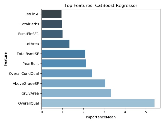
Feature Importance
Finally, the models can be scrutinized to determine which features are the most and least important in predicting the sales price and which do not contribute at all. Thus, the features that sell a house can be determined.
This article is a great summary of how to determine the feature importance of a model. For the most part, the feature importance can be used determined two different ways:
- Model based
- For Linear regression, this simply is the weights (or coefficients) from the fitted model. After the model has been fit, the weights are available via
model.coef_ - For Random Forests, XGBoost, and CatBoost models, a the importance values are all available via
model.feature_importances_
- For Linear regression, this simply is the weights (or coefficients) from the fitted model. After the model has been fit, the weights are available via
- Analyzing permutations of the data
- SKLearn contains permutation_importance which is functionality that determines the feature importance by analyzing how much the model score is impacted by randomly changing a features values. Permutation importance can be used on any model, including neural networks.
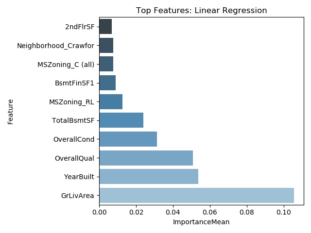
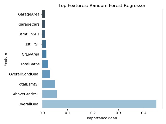
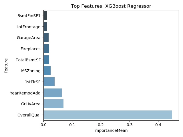
Below are graphs of the top ten most important features for the linear regression, random forest, XGBoost, and CatBoost models. It should be noted that degree of importance and the selected features are different among the models.
Sample Results
Below are some predictions made by the CatBoost model on the training dataset. Note that most features were used during model training but only the ten most important (found in the previous section) have been listed.
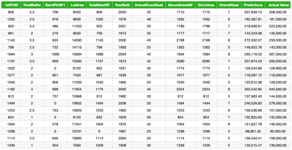
From the table, we can see that some predictions are very close to the actual value. A small percentage of the predictions are off but are still within an acceptable range.
Code
All of the code is available here.
No Comments