This is originally a Kaggle problem where the task is:
to build a predictive model that answers the question: “what sorts of people were more likely to survive?” using passenger data (ie name, age, gender, socio-economic class, etc).
The data is broken into train and test sets in a ratio of approximately 68 to 32 percent respectively with the following features:
- survival: if the passenger survived; 0 = No, 1 = Yes. This is what we are trying to predict
- pclass: ticket class; 1 = 1st, 2 = 2nd, 3 = 3rd
- sex: the gender of the passenger (male/female)
- age: age in years
- sibsp: number of siblings / spouses aboard the Titanic
- parch: number of parents / children aboard the Titanic
- ticket: Ticket number
- fare: Passenger fare
- cabin: Cabin number
- embarked: Port of Embarkation (or where the person boarded); C = Cherbourg, Q = Queenstown, S = Southampton
Getting Started
First we need to load the training data to see what we have…
import numpy as np
import pandas as pd
import matplotlib.pyplot as plt

# note the raw... this is the untouched data.
rawTrainingData = pd.read_csv ('train.csv')
rawTestData     = pd.read_csv ('test.csv')

# view the first few lines
rawTrainingData.head ()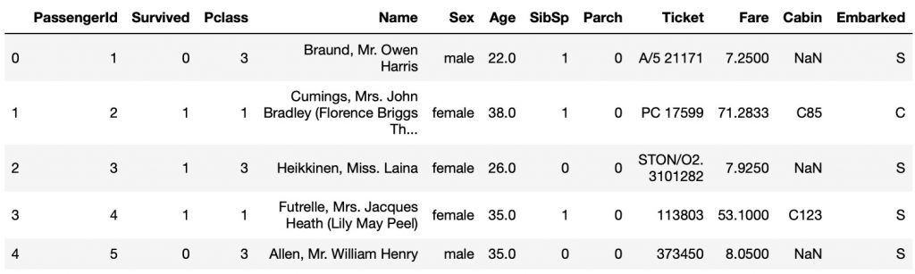
Next we check the range of values:
rawTrainingData.describe ()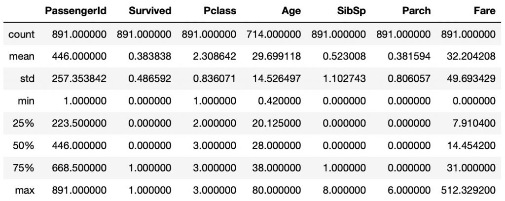
A few things to note: the average survival rate was 38.4% and the average ticket price was 32 pounds.
Look if any data is missing…
rawTrainingData.info ()

<class 'pandas.core.frame.DataFrame'>
RangeIndex: 891 entries, 0 to 890
Data columns (total 12 columns):
PassengerId    891 non-null int64
Survived       891 non-null int64
Pclass         891 non-null int64
Name           891 non-null object
Sex            891 non-null object
Age            714 non-null float64
SibSp          891 non-null int64
Parch          891 non-null int64
Ticket         891 non-null object
Fare           891 non-null float64
Cabin          204 non-null object
Embarked       889 non-null object
dtypes: float64(2), int64(5), object(5)
memory usage: 83.7+ KB
rawTestData.info ()
<class 'pandas.core.frame.DataFrame'>
RangeIndex: 418 entries, 0 to 417
Data columns (total 11 columns):
PassengerId 418 non-null int64
Pclass 418 non-null int64
Name 418 non-null object
Sex 418 non-null object
Age 332 non-null float64
SibSp 418 non-null int64
Parch 418 non-null int64
Ticket 418 non-null object
Fare 417 non-null float64
Cabin 91 non-null object
Embarked 418 non-null object
dtypes: float64(2), int64(4), object(5)
memory usage: 36.0+ KBMost things look ok except Age, Cabin, Fare, and Embarked are missing some elements.
Looking at the Data…
Cabin
rawTrainingData['Cabin'].value_counts ()

G6             4
B96 B98        4
C23 C25 C27    4
E101           3
F2             3
              ..
B94            1
E50            1
C111           1
C90            1
D47            1
Name: Cabin, Length: 147, dtype: int64
There is a lot of missing Cabin values. Also there is no noticeable pattern. Hence it will be removed/dropped from the dataset.
Age
First plot the age distribution…
plt.figure ()
plt.hist (rawTrainingData['Age'])
plt.show ()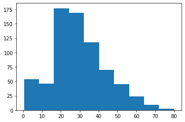
Since the age isn’t a nice normal distribution, we shall use the median to fill in the missing values.
rawTrainingData['Age'].median ()Fare
First we shall plot the data…
plt.figure ()
plt.hist (rawTrainingData['Fare'], bins=30)
plt.show ()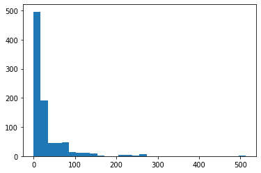
From the distribution and some experiments, the fares can be put into three different ranges… low, medium, and high.
pd.cut (rawTrainingData['Fare'], [0, 10, 25, 1000]).value_counts()

(25, 1000]    334
(0, 10]       321
(10, 25]      221
Name: Fare, dtype: int64
Embarked
Look at what it consists of…
rawTrainingData['Embarked'].value_counts()

S    644
C    168
Q     77
Name: Embarked, dtype: int64
Look at the rows with the missing values to try to make sense of things…
rawTrainingData[rawTrainingData['Embarked'].isna()]
There is something funny with this… both had the same ticket number, stayed in the same room, one was french and married, the other was single and english. Perhaps it is best to drop these two rows.
Sex
Looking at the values we see that it is easy enough to convert to a numeric value…
rawTrainingData['Sex'].value_counts()

male      577
female    314
Name: Sex, dtype: int64
Ticket
There seems to be some repetition in tickets…
rawTrainingData['Ticket'].value_counts()

1601                 7
CA. 2343             7
347082               7
CA 2144              6
3101295              6
                    ..
A.5. 18509           1
STON/O 2. 3101292    1
3101277              1
345778               1
PC 17475             1
Name: Ticket, Length: 681, dtype: int64
Hence, we will try to group the tickets together if possible using…
rawTrainingData.groupby("Ticket")["Ticket"].count()Name
From the Names we can extract some titles…
rawTrainingData['Name']

0                                Braund, Mr. Owen Harris
1      Cumings, Mrs. John Bradley (Florence Briggs Th...
2                                 Heikkinen, Miss. Laina
3           Futrelle, Mrs. Jacques Heath (Lily May Peel)
4                               Allen, Mr. William Henry
                             ...
886                                Montvila, Rev. Juozas
887                         Graham, Miss. Margaret Edith
888             Johnston, Miss. Catherine Helen "Carrie"
889                                Behr, Mr. Karl Howell
890                                  Dooley, Mr. Patrick
Name: Name, Length: 891, dtype: object
titles = {'Mr.': 0, 'Mrs.': 0, 'Miss.': 0, 'Master.': 0, 'Important': 0, 'Other': 0}
for i, name in enumerate (rawTrainingData['Name']):
nameTokens = name.split (' ')
if 'Mr.' in nameTokens:
titles['Mr.'] = titles['Mr.'] + 1
elif 'Mrs.' in nameTokens or 'Mme.' in nameTokens or 'Ms.' in nameTokens:
titles['Mrs.'] = titles['Mrs.'] + 1
elif 'Miss.' in nameTokens or 'Mlle.' in nameTokens:
titles['Miss.'] = titles['Miss.'] + 1
elif 'Master.' in nameTokens:
titles['Master.'] = titles['Master.'] + 1
elif 'Dr.' in nameTokens or 'Capt' in nameTokens or 'Col' in nameTokens or \
'Major' in nameTokens or 'Rev.' in nameTokens:
titles['Important'] = titles['Important'] + 1
else: # Sir, Lady, Countess, Jonkheer, and Don
titles['Other'] = titles['Other'] + 1
titles
{'Mr.': 517,
'Mrs.': 127,
'Miss.': 184,
'Master.': 40,
'Important': 13,
'Other': 10}Transforming the Data…
We shall make a function that will transform the data. It can be used for both the test and train sets. For now we are just one-hot encoding the categorical variables to get a baseline set of results.
def TransformData (dataset):
    # Drop for now drop cabin, name, and ticket... in the future we will might try to use them
    transformedDataset = dataset.drop (['Cabin', 'Name', 'Ticket'], axis=1)

    # Drop NA rows... looking at the embarked column...
    transformedDataset.dropna (axis=0, subset=['Embarked'], inplace=True)

    # Fill any missing ages with the median
    transformedDataset['Age'].fillna (transformedDataset['Age'].median(), inplace=True)

    # Fill any missing fares with the median
    transformedDataset['Fare'].fillna (transformedDataset['Fare'].median(), inplace=True)

    # One hot encode of the PClass column
    one_hot = pd.get_dummies (transformedDataset['Pclass'], prefix='PClass')
    transformedDataset.drop (['Pclass'], axis=1, inplace=True)
    transformedDataset = transformedDataset.join (one_hot)

    # One hot encode of the Embarked column
    one_hot = pd.get_dummies (transformedDataset['Embarked'], prefix='Embarked')
    transformedDataset.drop (['Embarked'], axis=1, inplace=True)
    transformedDataset = transformedDataset.join (one_hot)

    # One hot encode of the Sex column
    one_hot = pd.get_dummies (transformedDataset['Sex'], prefix='Sex')
    transformedDataset.drop (['Sex'], axis=1, inplace=True)
    transformedDataset = transformedDataset.join (one_hot)

    return transformedDataset
Modeling…
A few different models will be used:
- Support Vector Classifier
- Random Forest Classifier
- Logistic Regression
- Extreme Gradient Boosting (or XGBoost)
The idea is to try a few models and compare the results give a final result.
from sklearn.svm import SVC
from sklearn.ensemble import RandomForestClassifier
from sklearn.linear_model import LogisticRegression
import xgboost as xgb
To test for the accuracy of the model, we will average the cross_val_score:
from sklearn.model_selection import cross_val_scoreThe following is how the models are computed…
# make xTrain and yTrain data...
cleanedTrainingData = TransformData (rawTrainingData)
yTrain = cleanedTrainingData ['Survived']
xTrain = cleanedTrainingData.drop (['Survived', 'PassengerId'], axis=1)
svm_clf = SVC (gamma="auto")
svm_clf.fit (xTrain, yTrain)
svm_scores = cross_val_score(svm_clf, xTrain, yTrain, cv=10)
print (svm_scores.mean())
rf_clf = RandomForestClassifier (random_state=0)
rf_clf.fit (xTrain, yTrain)
rf_scores = cross_val_score (rf_clf, xTrain, yTrain, cv=10)
print (rf_scores.mean())
logit_clf = LogisticRegression(random_state=0, solver='lbfgs', max_iter=10000)
logit_clf.fit (xTrain, yTrain)
logit_scores = cross_val_score (logit_clf, xTrain, yTrain, cv=10)
print (logit_scores.mean())
model = xgb.XGBClassifier()
model.fit (xTrain, yTrain)
xgbScores = cross_val_score (model, xTrain, yTrain, cv=10)
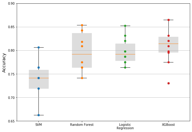
print (xgbScores.mean())Results so far… the mean accuracy score based on the training data was:
- SVC: 73.2%
- Random Forest: 79.8%
- Logistic Regression: 79.9%
- XGBoost: 81.1%
Below are box-graphs of the results… the random forest, logistic regression, and xgboost are all good candidates for improvement. The box plots show ten different accuracy scores from the training data during the cross validation process, along with the median, and first and third quartiles.
Improving the Model…
Things are ok but can perhaps can be improved. We shall try to improve the data a bit…
- use the names to have titles
- bin the fares and ages
- classify the number of people someone is travelling with
- use the ticket groupings
The new transform data function becomes:
def TransformData_V2 (dataset):

    # Drop for now drop cabin, name, and ticket... in the future we will might try to use them
    transformedDataset = dataset.drop (['Cabin'], axis=1)

    transformedDataset['Title'] = 0
    for i, name in enumerate (transformedDataset['Name']):
        nameTokens = name.split (' ')
        if 'Mr.' in nameTokens:
            transformedDataset.iloc [i, transformedDataset.columns.get_loc('Title')] = 1

        elif 'Mrs.' in nameTokens or 'Mme.' in nameTokens or 'Ms.' in nameTokens:
            transformedDataset.iloc [i, transformedDataset.columns.get_loc('Title')] = 2

        elif 'Miss.' in nameTokens or 'Mlle.' in nameTokens:
            transformedDataset.iloc [i, transformedDataset.columns.get_loc('Title')] = 3

        elif 'Master.' in nameTokens:
            transformedDataset.iloc [i, transformedDataset.columns.get_loc('Title')] = 4

        elif 'Dr.' in nameTokens or 'Capt' in nameTokens or 'Col' in nameTokens or \
             'Major' in nameTokens or 'Rev.' in nameTokens:
            transformedDataset.iloc [i, transformedDataset.columns.get_loc('Title')] = 5

        else: # Sir, Lady, Countess, Jonkheer, and Don
            transformedDataset.iloc [i, transformedDataset.columns.get_loc('Title')] = 6

    transformedDataset.drop (['Name'], axis=1, inplace=True)
    one_hot = pd.get_dummies (transformedDataset['Title'], prefix='Title')
    transformedDataset.drop (['Title'], axis=1, inplace=True)
    transformedDataset = transformedDataset.join (one_hot)

    transformedDataset['TicketCount'] = transformedDataset.groupby('Ticket')['Ticket'].transform('count')
    transformedDataset.drop (['Ticket'], axis=1, inplace=True)

    transformedDataset['FamSize'] = transformedDataset['SibSp'] + transformedDataset['Parch']
    transformedDataset['Single'] = transformedDataset['FamSize'].map(lambda s: 1 if s == 1 else 0)
    transformedDataset['SmallFamily'] = transformedDataset['FamSize'].map(lambda s: 1 if 2 <= s <= 4 else 0)
    transformedDataset['LargeFamily'] = transformedDataset['FamSize'].map(lambda s: 1 if 5 <= s else 0)

    transformedDataset = transformedDataset.drop (['SibSp', 'Parch'], axis=1)

    # Drop NA rows... looking at the embarked column...
    transformedDataset.dropna (axis=0, subset=['Embarked'], inplace=True)

    # Fill any missing ages with the median
    transformedDataset['Age'].fillna (transformedDataset['Age'].median(), inplace=True)
    ageGroups = pd.cut (transformedDataset['Age'], bins=[0,15,30,45,60,100], labels=['A', 'B', 'C', 'D', 'E'])
    transformedDataset.insert (5, 'AgeGroup', ageGroups)
    one_hot = pd.get_dummies (transformedDataset['AgeGroup'], prefix='AgeGroup')
    transformedDataset.drop (['AgeGroup'], axis=1, inplace=True)
    transformedDataset = transformedDataset.join (one_hot)

    # Fill any missing fares with the median
    transformedDataset['Fare'].fillna (transformedDataset['Fare'].median(), inplace=True)
    fareGroups = pd.cut (transformedDataset['Fare'], bins=[0,10,25,1000], labels=['A', 'B', 'C'])
    transformedDataset.insert (3, 'FareGroup', fareGroups)
    one_hot = pd.get_dummies (transformedDataset['FareGroup'], prefix='FareGroup')
    transformedDataset.drop (['FareGroup'], axis=1, inplace=True)
    transformedDataset = transformedDataset.join (one_hot)

    # One hot encode of the PClass column
    one_hot = pd.get_dummies (transformedDataset['Pclass'], prefix='PClass')
    transformedDataset.drop (['Pclass'], axis=1, inplace=True)
    transformedDataset = transformedDataset.join (one_hot)

    # One hot encode of the Embarked column
    one_hot = pd.get_dummies (transformedDataset['Embarked'], prefix='Embarked')
    transformedDataset.drop (['Embarked'], axis=1, inplace=True)
    transformedDataset = transformedDataset.join (one_hot)

    # One hot encode of the Sex column
    one_hot = pd.get_dummies (transformedDataset['Sex'], prefix='Sex')
    transformedDataset.drop (['Sex'], axis=1, inplace=True)
    transformedDataset = transformedDataset.join (one_hot)

    return transformedDataset
The results have improved a bit (hopefully the models are not overfitting the data)…
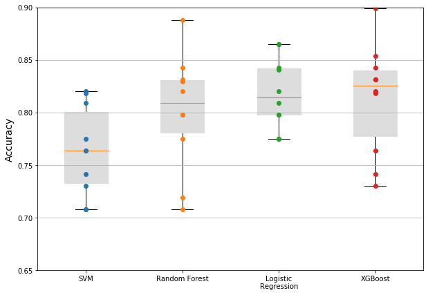
The average accuracy scores are now:
- SVC: 76.4%
- Random Forest: 80.1%
- Logistic Regression: 81.9%
- XGBoost: 81.3%
Tuning the Models…
Using grid search to find a better fitting model…
from sklearn.model_selection import GridSearchCV
# support vector machine...
parameter_grid = {
'C' : [ 1, 10, 100, 1000, 10000],
'kernel' : ['linear', 'rbf', 'sigmoid'],
'gamma': ['scale', 'auto']
}
svm_clf = SVC ()
grid_search = GridSearchCV (svm_clf,
scoring='accuracy',
param_grid=parameter_grid,
cv=3,
n_jobs=2,
verbose=1)
grid_search.fit (xTrain, yTrain)
model = grid_search.best_estimator_
parameters = grid_search.best_params_
print(f'Best score: {grid_search.best_score_}')
print(f'Best estimator: {grid_search.best_estimator_}')
# Find the best parameters for the random forest
parameter_grid = {
'max_depth' : [8, 10, 12],
'n_estimators': [10, 50, 100],
'max_features': ['sqrt'],
'min_samples_split': [2, 3, 10],
'min_samples_leaf': [1, 3, 10],
'bootstrap': [True, False] }
rf_clf = RandomForestClassifier(n_jobs=2)
grid_search = GridSearchCV (rf_clf,
scoring='accuracy',
param_grid=parameter_grid,
cv=3,
n_jobs=2,
verbose=1)
grid_search.fit (xTrain, yTrain)
model = grid_search.best_estimator_
parameters = grid_search.best_params_
print(f'Best score: {grid_search.best_score_}')
print(f'Best estimator: {grid_search.best_estimator_}')
# Find the best parameters for logit classifier
parameter_grid = {
'C' : [1e-4, 1e-3, 1e-2, 1e-1, 1, 10, 100] }
logit_clf = LogisticRegression(random_state=0, solver='lbfgs', max_iter=10000, n_jobs=2)
grid_search = GridSearchCV (logit_clf,
scoring='accuracy',
param_grid=parameter_grid,
cv=3,
n_jobs=2,
verbose=1)
grid_search.fit (xTrain, yTrain)
model = grid_search.best_estimator_
parameters = grid_search.best_params_
print(f'Best score: {grid_search.best_score_}')
print(f'Best estimator: {grid_search.best_estimator_}')
# xgboost...
parameter_grid = {
'max_depth' : [7, 8, 9],
'max_delta_step': [1],
'n_estimators': [20, 40, 60, 80],
'colsample_bylevel': [0.8, 0.9, 1.0],
'colsample_bytree': [0.6, 0.8, 1.0],
'subsample': [0.3, 0.4, 0.5, 0.6],
}
xgb_clf = xgb.XGBClassifier()
grid_search = GridSearchCV (xgb_clf,
scoring='accuracy',
param_grid=parameter_grid,
cv=3,
n_jobs=2,
verbose=1)
grid_search.fit (xTrain, yTrain)
model = grid_search.best_estimator_
parameters = grid_search.best_params_
print(f'Best score: {grid_search.best_score_}')
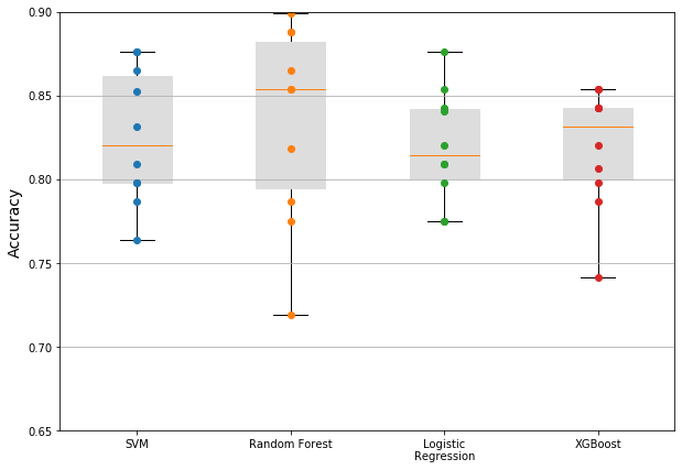
print(f'Best estimator: {grid_search.best_estimator_}')From the grid search we were able to produce the following results…
- SVM: 82.6%
- Random Forest: 83.5%
- Logistic Regression: 82.0%
- XGBoost: 81.9%
Finally Test out the results on Kaggle…
Using the final tuned models on the test set which were then verified with kaggle. First the code used to generate the kaggle output was:
cleanedTestingData = TransformData_V2 (rawTestData)
xTest = cleanedTestingData.drop (['PassengerId'], axis=1)

yPred_svm   = svm_clf.predict (xTest)
yPred_logit = logit_clf.predict (xTest)
yPred_rf    = rf_clf.predict (xTest)
yPred_xgb   = xgb_clf.predict (xTest)

output = pd.DataFrame({'PassengerId': cleanedTestingData.PassengerId, 'Survived': yPred_svm})
output.to_csv('sub_svm_tuned.csv', index=False)

output = pd.DataFrame({'PassengerId': cleanedTestingData.PassengerId, 'Survived': yPred_logit})
output.to_csv('sub_logit_tuned.csv', index=False)

output = pd.DataFrame({'PassengerId': cleanedTestingData.PassengerId, 'Survived': yPred_rf})
output.to_csv('sub_rf_tuned.csv', index=False)

output = pd.DataFrame({'PassengerId': cleanedTestingData.PassengerId, 'Survived': yPred_xgb})
output.to_csv('sub_xgb_tuned.csv', index=False)
A few noticeable things from the results:
- All the steps do improve the results on the training data, however this might be a sign of overfitting
- Logistic regression was the overall winner (78%) with how the data was transformed.
- It seems that the random forest and xgboost classifiers can easily overfit the data.
| Support Vector Classifier |
Random Forest |
Logistic Regression |
XGBoost | |
|---|---|---|---|---|
| Plain Model | 73.2% | 79.8% | 79.9% | 81.1% |
| Model with new Features |
76.4% | 80.1% | 81.9% | 81.3% |
| Tuned Model | 82.6% | 83.5% | 82.0% | 81.9% |
| Testing Data | 77.03% | 76.56% | 77.99% | 71.5% |
This problem was more of a learning exercise so instead of spending more time on this problem to try to improve the score on the testing set, perhaps its better to move on to the next problem.
Code…
All the code is available here as a Jupyter notebook.
No Comments