I have to admit that I wasn’t the biggest fan of the Koch curve and/or snowflake object. Perhaps they were too simple, since they are located at the front of a fractal book and the cool stuff is usually located towards the back. Being winter I thought that this project was an appropriate way to try to get myself in a more festive mood.
The basics in constructing a Koch curve is to first start with a straight line, and then replace the middle third with two segments of the same length. This process is repeated in a recursive manor on the remaining line segments. By connecting three Koch curves end to end, results in a snowflake like object (or anti snowflake/island). One interesting property of the Koch snowflake is that it have infinite perimeter but finite area.
In this project, a few implementations of the Koch snowflake were made including those using L systems, IFSs, along with various tilings.
L System
The Koch curve and snowflake can be described by the following L-system:
\begin{aligned}
\mathsf{Initial\ Axiom} :&\ F + + F + + F \\
\mathsf{Rule(s)} :&\ F \mapsto F-F++F-F \\
\mathsf{Angle} :&\ 60^\circ
\end{aligned}
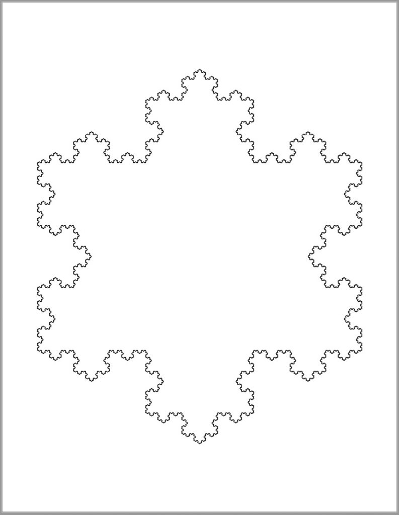
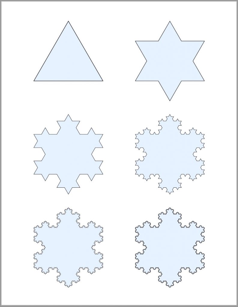
By recursively applying the L system, we can generate the classic Koch snowflake. Below we have the results after 7 iterations on the left, and the first 5 iterations (along with the initial state) on the right.
IFS
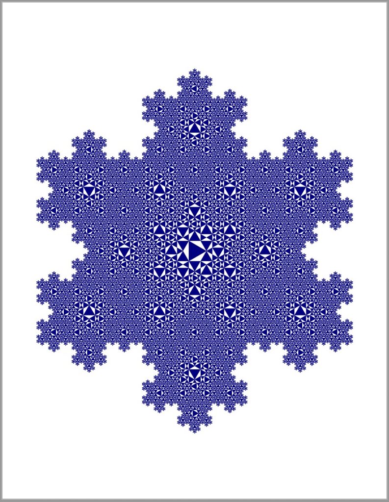
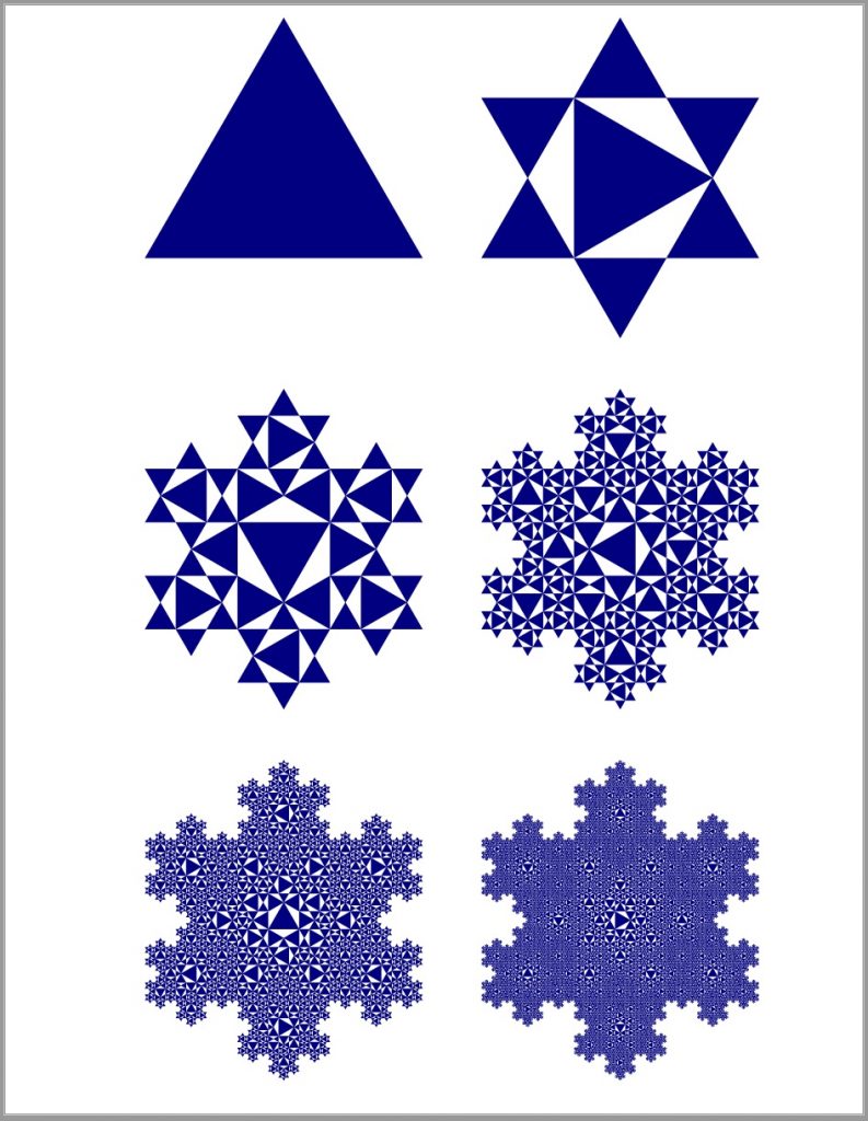
Two different iterated function systems (or IFS) were used to create space filling curves based on the Koch snowflake. Both were taken from the following page, however there are some minor errors with some of the values so I have listed all of the transformations that I used below.
IFS 1
The following is the set of transformations for the first IFS (or simply IFS 1). For each iteration, all 7 transforms are applied to each point in the object. Note that several new points are created each cycle and those need to be transformed with the next iteration as well.
\begin{aligned}
t_1 \left( \begin{array}{c} x \\ y\end{array} \right) &=
\left( \begin{array}{cc} -\frac{1}{6} & \frac{\sqrt{3}}{6} \\ \vphantom{a} \\ -\frac{\sqrt{3}}{6} & -\frac{1}{6}\end{array} \right) \left( \begin{array}{c} x \\
y\end{array} \right) + \left( \begin{array}{c} \frac{1}{6} \\ \vphantom{a} \\ \frac{\sqrt{3}}{6} \end{array} \right) \\
\vphantom{a} \\
t_2 \left( \begin{array}{c} x \\ y\end{array} \right) &= \left( \begin{array}{cc} \frac{1}{6} & -\frac{\sqrt{3}}{6} \\ \vphantom{a} \\ \frac{\sqrt{3}}{6} & \frac{1}{6}\end{array} \right) \left( \begin{array}{c} x \\ y\end{array} \right) + \left( \begin{array}{c} \frac{1}{6} \\ \vphantom{a} \\ \frac{\sqrt{3}}{6} \end{array} \right) \\
\vphantom{a} \\
t_3 \left( \begin{array}{c} x \\ y\end{array} \right) &= \left( \begin{array}{cc} \frac{1}{3} & 0 \\ \vphantom{a} \\ 0 & \frac{1}{3}\end{array} \right) \left( \begin{array}{c} x \\ y\end{array} \right) + \left( \begin{array}{c} \frac{1}{3} \\ \vphantom{a} \\ \frac{\sqrt{3}}{3} \end{array} \right) \\
\vphantom{a} \\
t_4 \left( \begin{array}{c} x \\ y\end{array} \right) &= \left( \begin{array}{cc} \frac{1}{6} & \frac{\sqrt{3}}{6} \\ \vphantom{a} \\ -\frac{\sqrt{3}}{6} & \frac{1}{6}\end{array} \right) \left( \begin{array}{c} x \\ y\end{array} \right) + \left( \begin{array}{c} \frac{2}{3} \\ \vphantom{a} \\ \frac{\sqrt{3}}{3} \end{array} \right) \\
\vphantom{a} \\
t_5 \left( \begin{array}{c} x \\ y\end{array} \right) &= \left( \begin{array}{cc} \frac{1}{2} & -\frac{\sqrt{3}}{6} \\ \vphantom{a} \\ \frac{\sqrt{3}}{6} & \frac{1}{2}\end{array} \right) \left( \begin{array}{c} x \\ y\end{array} \right) + \left( \begin{array}{c} \frac{1}{3} \\ \vphantom{a} \\ 0 \end{array} \right) \\
\vphantom{a} \\
t_6 \left( \begin{array}{c} x \\ y\end{array} \right) &= \left( \begin{array}{cc} -\frac{1}{3} & 0 \\ \vphantom{a} \\ 0 & -\frac{1}{3}\end{array} \right) \left( \begin{array}{c} x \\ y\end{array} \right) + \left( \begin{array}{c} \frac{2}{3} \\ \vphantom{a} \\ 0 \end{array} \right) \\
\vphantom{a} \\
t_7 \left( \begin{array}{c} x \\ y\end{array} \right) &= \left( \begin{array}{cc} \frac{1}{3} & 0 \\ \vphantom{a} \\ 0 & \frac{1}{3}\end{array} \right) \left( \begin{array}{c} x \\ y\end{array} \right) + \left( \begin{array}{c} \frac{2}{3} \\ \vphantom{a} \\ 0 \end{array} \right) \\
\end{aligned}
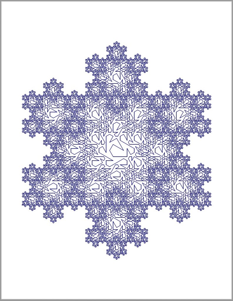
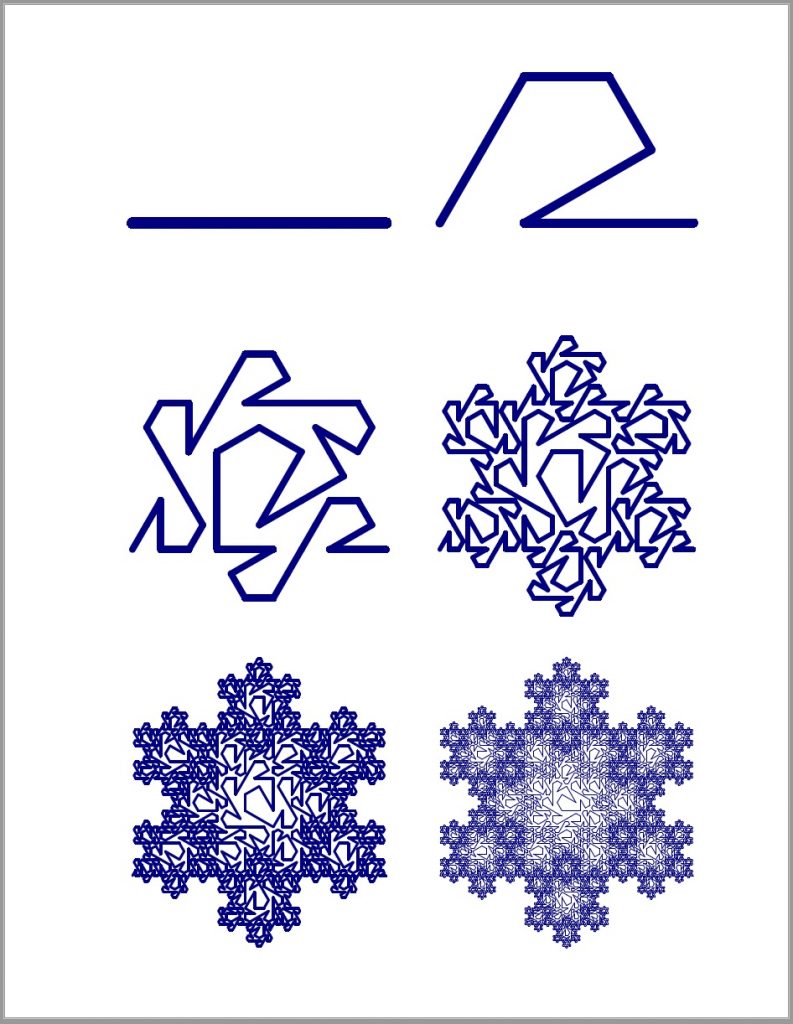
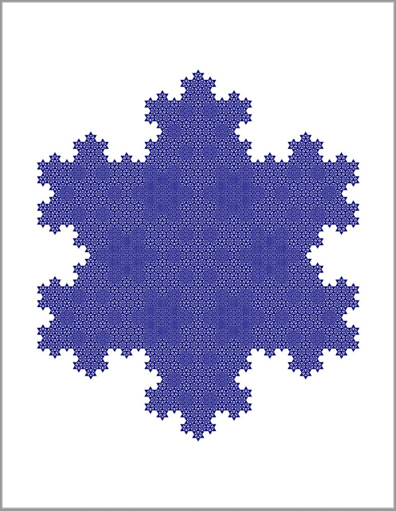
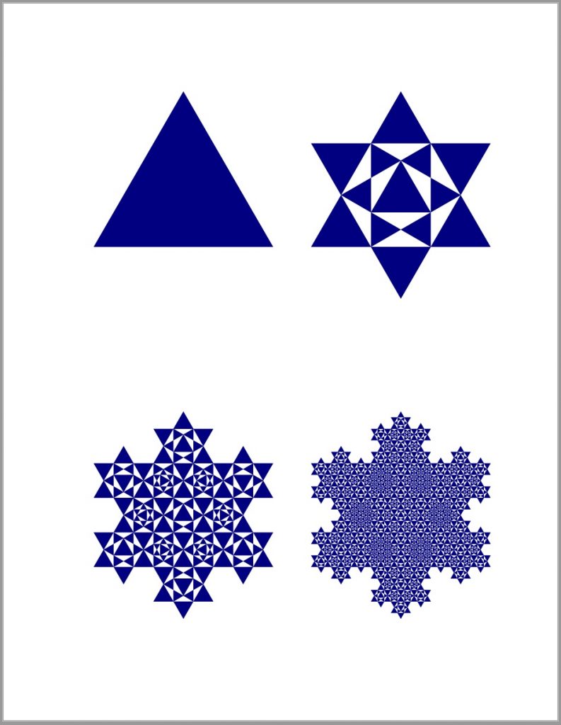
Using the above IFS on a line segment and an equilateral triangle the following results were produced. Note that the left images are the results after 5 iterations, and the right show the first 5 iterations along with the initial state.
IFS 2
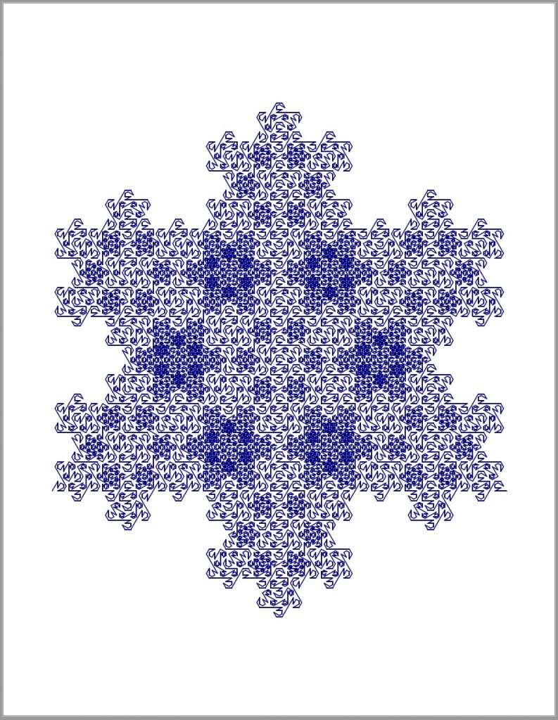
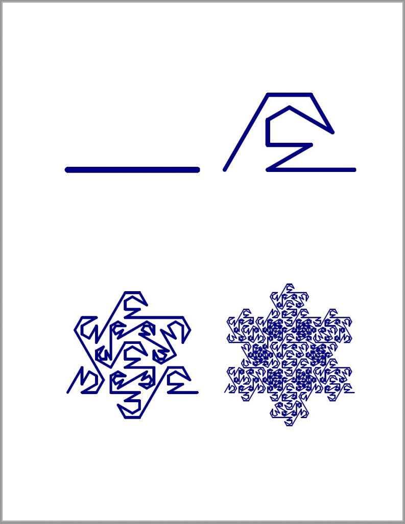
IFS 2 is based on the transformations from IFS1 except for t_5. That particular transform is replaced with 7 other transforms that are listed below to give a total of 13. These extra transforms make the results slightly more interesting.
\begin{aligned}
t_{5a} \left( \begin{array}{c} x \\ y\end{array} \right) &=
\left( \begin{array}{cc} -\frac{1}{6} & -\frac{\sqrt{3}}{18} \\
\vphantom{a} \\ \frac{\sqrt{3}}{18} & -\frac{1}{6}\end{array} \right) \left( \begin{array}{c} x \\ y\end{array} \right) + \left( \begin{array}{c} \frac{5}{6} \\ \vphantom{a} \\ \frac{\sqrt{3}}{6} \end{array} \right) \\
\vphantom{a} \\
t_{5b} \left( \begin{array}{c} x \\ y\end{array} \right) &= \left( \begin{array}{cc} -\frac{1}{6} & -\frac{\sqrt{3}}{18} \\
\vphantom{a} \\ \frac{\sqrt{3}}{18} & -\frac{1}{6}\end{array} \right) \left( \begin{array}{c} x \\ y\end{array} \right) + \left( \begin{array}{c} \frac{1}{2} \\ \vphantom{a} \\ \frac{5\sqrt{3}}{18} \end{array} \right) \\
\vphantom{a} \\
t_{5c} \left( \begin{array}{c} x \\ y\end{array} \right) &= \left( \begin{array}{cc} \frac{1}{6} & -\frac{\sqrt{3}}{18} \\
\vphantom{a} \\ \frac{\sqrt{3}}{18} & \frac{1}{6}\end{array} \right) \left( \begin{array}{c} x \\ y\end{array} \right) + \left( \begin{array}{c} \frac{1}{3} \\ \vphantom{a} \\ \frac{2\sqrt{3}}{9} \end{array} \right) \\
\vphantom{a} \\
t_{5d} \left( \begin{array}{c} x \\ y\end{array} \right) &= \left( \begin{array}{cc} 0 & -\frac{\sqrt{3}}{9} \\
\vphantom{a} \\ \frac{\sqrt{3}}{9} & 0 \end{array} \right) \left( \begin{array}{c} x \\ y\end{array} \right) + \left( \begin{array}{c} \frac{1}{3} \\ \vphantom{a} \\ \frac{\sqrt{3}}{9} \end{array} \right) \\
\vphantom{a} \\
t_{5e} \left( \begin{array}{c} x \\ y\end{array} \right) &= \left( \begin{array}{cc} \frac{1}{3} & 0 \\
\vphantom{a} \\ 0 & \frac{1}{3} \end{array} \right) \left( \begin{array}{c} x \\ y\end{array} \right) + \left( \begin{array}{c} \frac{1}{3} \\ \vphantom{a} \\ \frac{\sqrt{3}}{9} \end{array} \right) \\
\vphantom{a} \\
t_{5f} \left( \begin{array}{c} x \\ y\end{array} \right) &= \left( \begin{array}{cc} -\frac{1}{6} & \frac{\sqrt{3}}{18} \\
\vphantom{a} \\ -\frac{\sqrt{3}}{18} & -\frac{1}{6} \end{array} \right) \left( \begin{array}{c} x \\ y\end{array} \right) + \left( \begin{array}{c} \frac{2}{3} \\ \vphantom{a} \\ \frac{\sqrt{3}}{9} \end{array} \right) \\
\vphantom{a} \\
t_{5g} \left( \begin{array}{c} x \\ y\end{array} \right) &= \left( \begin{array}{cc} \frac{1}{6} & -\frac{\sqrt{3}}{18} \\
\vphantom{a} \\ \frac{\sqrt{3}}{18} & \frac{1}{6} \end{array} \right) \left( \begin{array}{c} x \\ y\end{array} \right) + \left( \begin{array}{c} \frac{1}{3} \\ \vphantom{a} \\ 0 \end{array} \right)
\end{aligned}
Just like with IFS 1, the results were generated using a line segment and an equilateral triangle. The left images are the results after 4 iterations, and the right show the first 3 iterations along with the initial state. Note that the extra transformations in the IFS really add to the size of the resulting figure. So figures of more than 5 iterations result in a very crowded image where fine details can not be easily resolved and so have been omitted.
Periodic Tiling
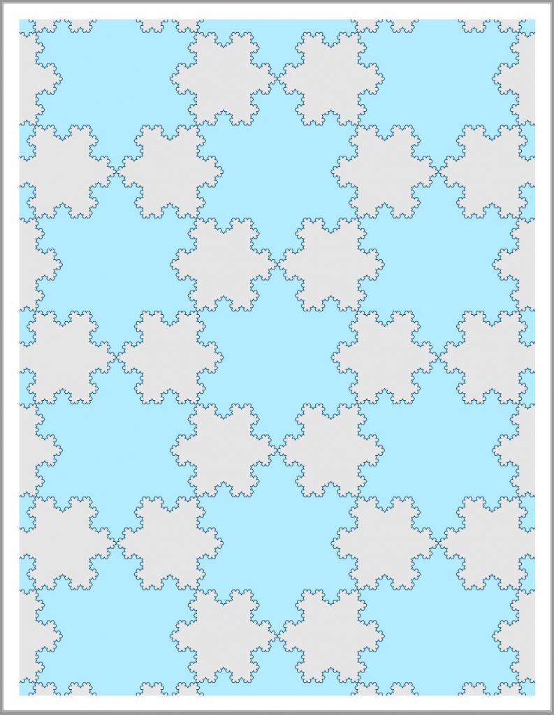
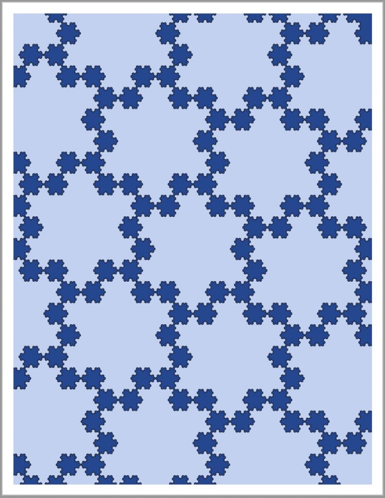
Sets of Koch snowflakes can be placed together in such a manor where a plane can be periodically tiled to give some visually appealing results. Quite often (but not always) it is possible to produce more snowflakes within the remaining space. For example, two such tiling transformations are:
\begin{aligned}
t_1 &= m \left(0, h\vphantom{\frac{1}{2}}\right) + n \left(w, \frac{1}{2}h\right) \\
t_2 &= m \left( \frac{2}{3}w, \frac{2}{3}h\right) + n \left( w, \frac{1}{6}h \right)
\end{aligned}
Where m and n are integers used to the place the snowflakes, and w and h are the width and height each unit. Using these two tiling transformations, the following results created where t_1 was used on the left and t_2 with those on the right. To emphasize the snowflakes created by the remaining space, the colour of the background was changed to grey and dark blue.
Recursive Tiling
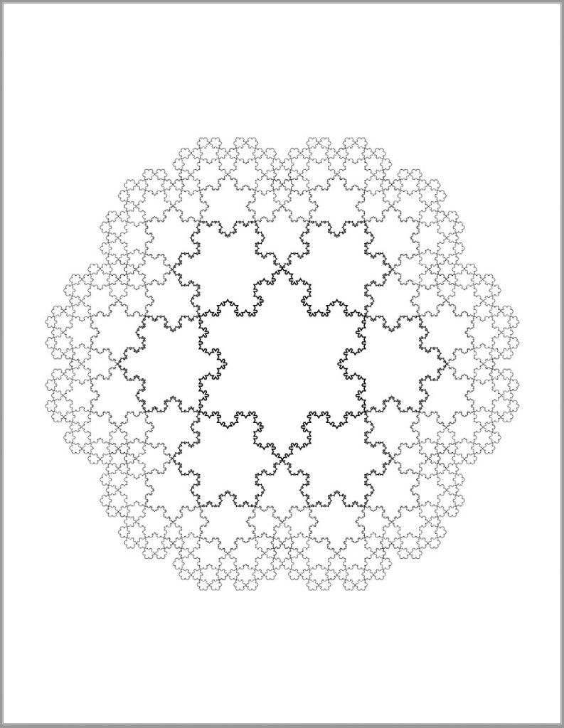
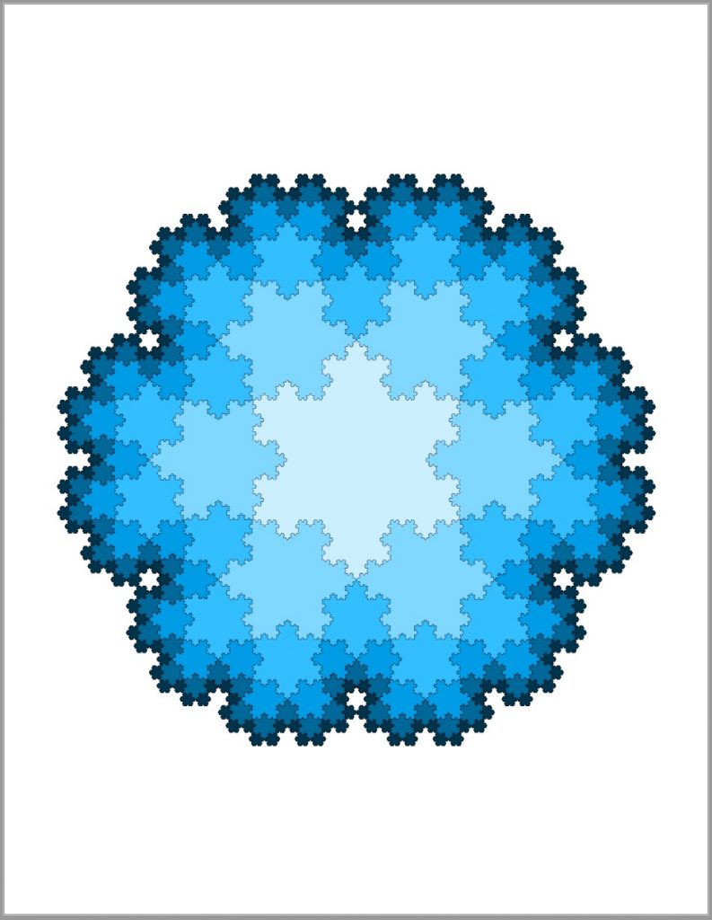
It is possible to recursively tile the Koch snowflake to achieve a rather nice and visually appealing result (I must admit that this is my favourite result of them all).
For each iteration, new snowflakes are drawn around an existing one at 60 degree intervals and placed so that their edges are coincident. Also at each step, the new results are scaled down by a factor of \sqrt{3} and rotated by 30 degrees. Below is the results after 5 recursive iterations (in both black & white and various shades of blue).
Code…
All of the code and output is available here.
Other Stuff…
During the investigation process, a few different Koch snowflake inspired links were discovered along the way. All of these were amusing in their own special way.
- These guys made a gigantic pecan pie based on the Koch snowflake. This is one of my most favourite projects ever. They even made their own oven to cook it.
- There are a variety of Koch curve inspired jewelry pieces out there, such as this one
- This wooden puzzle seems to be hours of fun. All the tilings listed above and more can be made.
- A few people over the years made 3D Koch snowflakes out of paper; like with this cool implementation or with this video
Fractals Postscript Winter
No Comments